semi合集-English.pdf - 第106页

SEMI E10-0304 E © SEMI 1986, 2004 20 R1-3.3.3 For a failure whose onset occu rs outside of the observation period , the portion of its repair time that occurs within the observation period is still coun ted in MTTR CT . …

SEMI E10-0304

R1-2.2.2 Unscheduled downtime state shall be tracked

for each module. Tracking of unscheduled downtime

state for the multi-path cluster tool as a whole is not

sufficient. A module cannot be in productive and

unscheduled downtime states at the same time. Each

contiguous instance of unscheduled downtime state for

a module is a module failure. Subsequent substate

events within the same instance of unscheduled

downtime state shall not to be counted as additional

failures.

R1-2.2.3 Scheduled downtime state shall be tracked for

each module. Tracking of scheduled downtime state

for the multi-path cluster tool as a whole is not

sufficient. A module cannot be in productive and

scheduled downtime states at the same time. Instances

of scheduled downtime shall not to be counted as

failures.

R1-2.2.4 Time in standby and engineering states shall

not be considered as either productive time, scheduled

downtime, or unscheduled downtime at the module

level. For the purpose of tracking multi-path cluster

tool states and calculating multi-path cluster tool and

process flow metrics, modules in these states are

considered as being in a neutral state.

R1-2.2.5 Non-scheduled time that is tracked for the

multi-path cluster tool as a whole is omitted from

operations time in calculating multi-path cluster tool

and process flow RAM metrics, as it is with the other

SEMI E10 metrics from the main body of the

specification. Non-scheduled time that is allocated to

some modules but not other modules, if any, shall be

handled differently, as follows.

R1-2.2.5.1 For new modules under installation that

have not yet been used for their intended function, those

modules shall be considered as non-existent in the

cluster-tool configuration.

R1-2.2.5.2 For installed modules that have been used,

non-scheduled time state shall be treated as a neutral

state.

R1-2.3 To calculate these metrics, an observation

period shall be defined and agreed upon by the user

and/or the supplier. Section A1-1.3 provides some

guidance on establishing the observation period time

needed to demonstrate a desired MTBF

at a given

confidence level.

R1-2.3.1 observation period time — elapsed calendar

time (e.g., weeks, months, quarters) observing and

tracking tool performance. No allowance is made for

the number of modules in a cluster tool.

R1-3 Total Failure Rate and Cluster-Tool Mean

Time to Repair

R1-3.1 Total Failure Rate (TFR) — total count of

module-level failure onsets, tracked according to the

requirements in Section R1-2, divided by the

observation period time. This metric characterizes the

frequency of repairs where failures on separate modules

are presumed to require independent repair actions.

TFR is an indicator of reliability and maintainability.

TFR is defined as:

TFR =

all modules

count of module failure onset events

observation

eriod time

NOTE 2: For different multi-path cluster tools with

comparable module failure rates, a multi-path cluster tool

with fewer modules is expected to have better performance

according to this metric than one with more modules.

However, the multi-path cluster tool with more modules may

have a better aggregate intended process flow uptime

(Uptime

CT-IPF

), as defined in Section R1-7.3.

R1-3.2 Cluster-Tool Mean Time to Repair (MTTR

)

— mean time to correct a module-level failure and

return the module to a condition where it can perform

its intended function; the sum of all repair time on all

modules (elapsed module time, not necessarily total

work-hours) incurred during a specified observation

period time (including equipment and process test time,

but not including maintenance delay downtime),

divided by the total number of failure onset events

during that period.

TTR

all modules

repair time

all modules

count of module failure onset events

NOTE 3: This is the same equation as MTTR for non-cluster

and single-path cluster tools. However, because a multi-path

cluster-tool may have repairs occurring simultaneously, the

sum of repair time is not constrained to the duration of the

observation period.

R1-3.3 For any module, a failure onset event is the first

chronological event of a contiguous instance of

unscheduled downtime. To ensure that over multiple

observation periods, neither failure onset events nor

repair time is ever double-counted, the following rules

shall be followed.

R1-3.3.1 Failure onset events that occur during the

observation period are counted in TFR and MTTR

regardless of when those failures are resolved.

R1-3.3.2 Failure onset events that occur before the

observation period are not counted in TFR and

MTTR

, even if those failures are not resolved until

during or after the observation period.

SEMI E10-0304

R1-3.3.3 For a failure whose onset occurs outside of

the observation period, the portion of its repair time that

occurs within the observation period is still counted in

MTTR

NOTE 4: These metrics also may be calculated for any multi-

module tool even if that tool is not a multi-path cluster tool.

For a system failure that arises from multiple module failures,

the additional severity of this case and the independence of

module repair efforts are reflected in this metric. For standard

evaluation of a non-multi-path cluster tool, however, the tool

is considered to be either entirely in the unscheduled

downtime state or not in the unscheduled downtime state.

R1-3.4 These metrics are not compatible with

approaches based on renewal cycle models where

uptime and downtime are assumed to be mutually

exclusive. As such, subsequent module failures may

occur even while failures are already in progress on

other modules. Other renewal cycle results (e.g., the

limiting probability of finding the system “up” (or

“down”) when approaching the system at random)

similarly may not apply.

R1-4 Temporal Mapping

R1-4.1 Temporal mapping provides an output state

history as a function of constituent input state histories.

For each event when at least one of the modules

changes state, the states of the process flows and/or

cluster tool may change. For the metrics in this related

information, cluster-tool and process-flow state

histories are generated as functions of module state

histories on an event-by-event basis in temporal, or

chronological, order. The metrics themselves are

calculated as functions of these output state histories.

For reference, this technique may be regarded as

generating a type of convolution of constituent state

models.

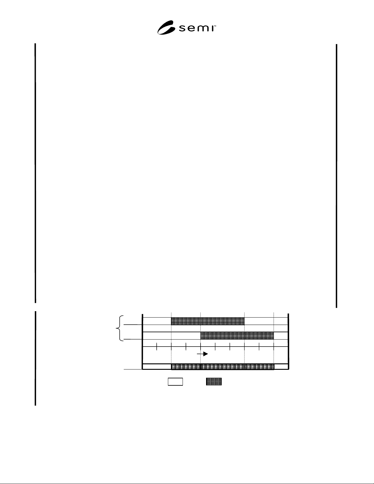
R1-4.2 Figure R1-1 presents an example of temporal

mapping. The constituent input states for two modules,

M1 and M2, are shown over the observation period t =

0 to t = 10. An output state is mapped temporally as a

function of the module states, where if either module is

“down” or both modules are “down,” the output state is

“down.” Note that transition events for the output state

history are the union set of the transition events for the

constituent input state histories.

R1-4.3 In a near-real-time tracking system, temporal

mapping may be performed as each event is generated

and received by the tracking system. Temporal

mapping also may be performed afterwards as a batch

process. Regardless, the logical process is the same.

Depending on the mapping to be performed, a different

logic function is applied at each input state transition

event to derive an output state value as a function of the

constituent input state values. Two specific temporal

mapping functions are used in metrics in this related

information:

R1-4.3.1 Process flow “up/scheduled downtime/

unscheduled downtime” states from module

“up/scheduled downtime/unscheduled downtime” states

as a function of supplier-defined and/or user-defined

process flows.

R1-4.3.2 Multi-path cluster tool “productive/neutral/

unscheduled downtime” as a standard function,

presented herein, of module “productive/not-

productive” states and process-flow “up/scheduled

downtime/unscheduled downtime” states.

NOTE 5: While it may be theoretically possible to model the

desired output states using Harel notation and modeling

concepts, output state complexity may be confounded by the

combinatorial nature of multi-path cluster tools and their

process flows. For this application, the temporal mapping

approach is much more straightforward.

100

time

Constituent

Input

States

Output

State

own

= Up

Figure R1-1

An Example Of Temporal Mapping

SEMI E10-0304

R1-5 Modeling Process Flows

R1-5.1 In order to evaluate multi-path cluster tool

availability and reliability, the set of process flows shall

be defined for the multi-path cluster tool. It is

important to differentiate between all the process flows

that are theoretically possible on a given multi-path

cluster tool configuration and those intended process

flows (IPF) that are actually intended for operational

use (i.e., performing its intended function). For

meaningful agreement between any two parties on the

metrics presented in this related information, first there

shall be documented agreement on the set of IPFs used

for evaluation, so that any analyst with the module state

histories can calculate the same values for the metrics.

First, the general case of “up/down” states for an IPF is

presented, and then later the distinction between

unscheduled downtime and total (i.e., scheduled and

unscheduled) downtime for an IPF is presented.

R1-5.2 An IPF “up/down” state is modeled as a

network flow through the modules that make up that

IPF. If there is “connectivity” through the IPF network,

then the IPF is “up;” otherwise it is “down.” The

modules in an IPF network have series and parallel

relationships that determine the connectivity through

the network. Mathematically, each module and each

IPF has a state value equal to 1 when the state is “up”

and 0 when the state is “down.” For example,

1, if module i is up

0, if module i is down

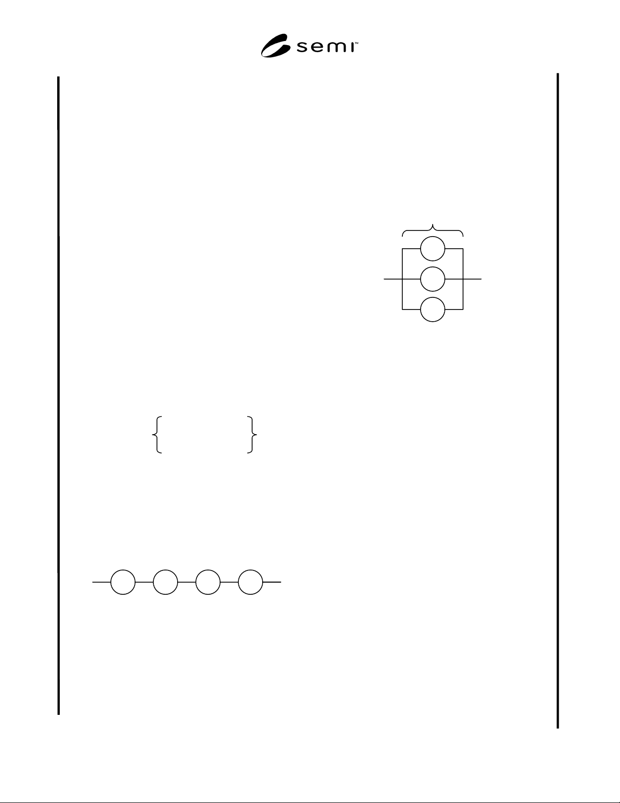
R1-5.3 The general process steps within an IPF have a

mutually serial relationship (i.e., if connectivity is not

possible through any single step, then connectivity is

not possible through the network). This is illustrated in

Figure R1-2. The IPF state value for serial constituents

is calculated as the product of the constituent state

values (e.g., IPF =

i=1 to 4

Si = S1 × S2 × S3

S4).

S1 S2 S3 S4

Figure R1-2

Serial Process Steps Within An IPF

R1-5.4 At any general process step, S

, the set of

alternative modules, Ai (if any are present), have a

mutually parallel relationship (i.e., if any one of the

alternative modules is up, then connectivity through

that step is still possible). This is illustrated in Figure

R1-3. The state value through this step is calculated as:

IPF = 1 -

i=1 to 3

(1 − Ai)

= 1 − [(1 − A1)

(1 − A2) × (1 − A3)]

If any alternative module is “up,” the expression in the

square brackets evaluates to zero, and the IPF state

value evaluates to 1, or “up.” If all of the alternative

modules are “down,” the expression in the square

brackets evaluates to 1, and the IPF state value

evaluates to 0, or “down.”

Figure R1-3

Parallel Alternative Modules At A Process Step

NOTE 6: In general network modeling, it is possible to have

complicated multi-constituent structures in parallel with other

multi-constituent structures. At the time of this writing, the

need for such structures in evaluating multi-path cluster tool

RAM is not anticipated. Therefore, this exposition is limited

to serial relationships amongst the process steps and single-

constituent parallel relationships for alternatives within any

one step. To model multi-path cluster tool systems that

exceed these limitations, the modeler is encouraged to consult

any text on the modeling of coherent systems for reliability.

R1-5.5 For almost all systems, there will be a subset of

modules that will appear in every IPF regardless of any

process differentiation, called the key group. The key

group includes support modules (e.g., transport, load

locks), common process modules that are used by every

IPF, and the platform itself. A key group may include

alternative modules such as multiple load locks or

multiple cooling stations. The key group’s relationship

to all IPFs is such that if the key group is down, all IPFs

are down. Therefore, the key group has a serial

relationship to each IPF. By modeling a key group and

leveraging it in calculations, substantial redundant

calculations are avoided. Furthermore, understanding

which modules belong to the key group also helps in

understanding and improving overall system reliability.

R1-5.6 Two examples are now presented to illustrate

how to model IPFs, including modeling of the key

group and of IPF state functions.