semi合集-English.pdf - 第111页

SEMI E10-0304 E © SEMI 1986, 2004 25 R1-5.6.2.8 The co at/develop system is likely to h ave several more IPFs defined essentially in the same manner as IPF 1 and IPF2, shown a bove. R1-5.7 Unscheduled Downtime versus Tot…

SEMI E10-0304

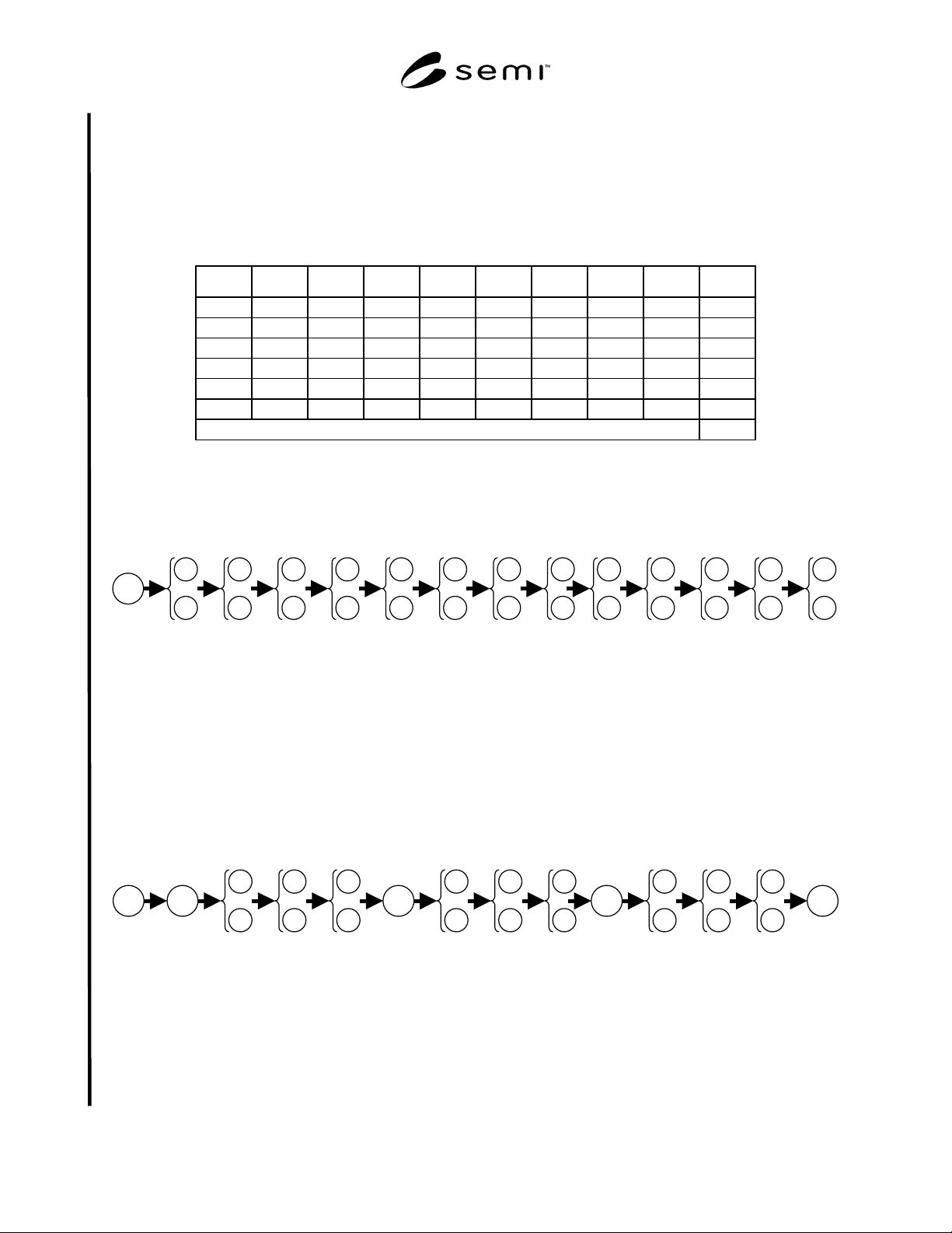
R1-5.6.2.2 The state value function for the key group is K = P

[1 − Π

i = 1 to 4

(1 − Li)] × Π

j=1 to 4

Rj, which can be

expanded to:

K = P × [1 − (1 − L1) × (1 − L2)

(1 − L3)

(1 − L4)]

R1-5.6.2.3 The equivalent truth table is shown in Table R1-3:

Table R1-3 Truth Table for State Function, Example 2

P L1 L2 L3 L4 R1 R2 R3 R4 K

0 any any any any any any any any 0

1 0 0 0 0 any any any any 0

any any any any any 0 any any any 0

any any any any any any 0 any any 0

any any any any any any any 0 any 0

any any any any any any any any 0 0

else 1

NOTE 7: This truth table emphasizes the subsets that bring the key group “down,” which are called minimum cut sets, rather

than the subsets that keep the key group “up,” called minimum path sets.

R1-5.6.2.4 IPF1 has 13 steps and each step has two alternative modules, as shown in Figure R1-10.

step 1

step 2

step 3

step 4

step 5

step 6

step 7

step 8

step 9

step 10

step 11

step 12

step 13

Figure R1-10

Module Configuration For IPF1, Example 2

R1-5.6.2.5 The state value function for IPF1 = K

i=1 to 13

[1 − (1 − PM

i,1

)

(1 − PM

i,2

)]. The equivalent truth

table is highly redundant and is therefore omitted.

R1-5.6.2.6 IPF2 has the same 13 steps as IPF1. However due to process matching issues, all units are restricted to a

single process module at steps 1, 5, 9, and 13, as shown in Figure R1-11.

step 1

step 2

step 3

step 4

step 5

step 6

step 7

step 8

step 9

step 10

step 11

step 12

step 13

Figure R1-11

Module Configuration For IPF2, Example 2

R1-5.6.2.7 The state value function for IPF2 = K

1,1

5,1

9,1

13,1

i={2-4, 6-8, 10-12}

[1 − (1 −

i,1

) × (1 − PM

i,2

)]

SEMI E10-0304

R1-5.6.2.8 The coat/develop system is likely to have

several more IPFs defined essentially in the same

manner as IPF1 and IPF2, shown above.

R1-5.7 Unscheduled Downtime versus Total Downtime

— In order to make a distinction between unscheduled

downtime and total downtime for an IPF, the IPF

function discussed thus far shall be executed twice:

once to determine an unscheduled downtime state and a

second time to determine a general downtime state.

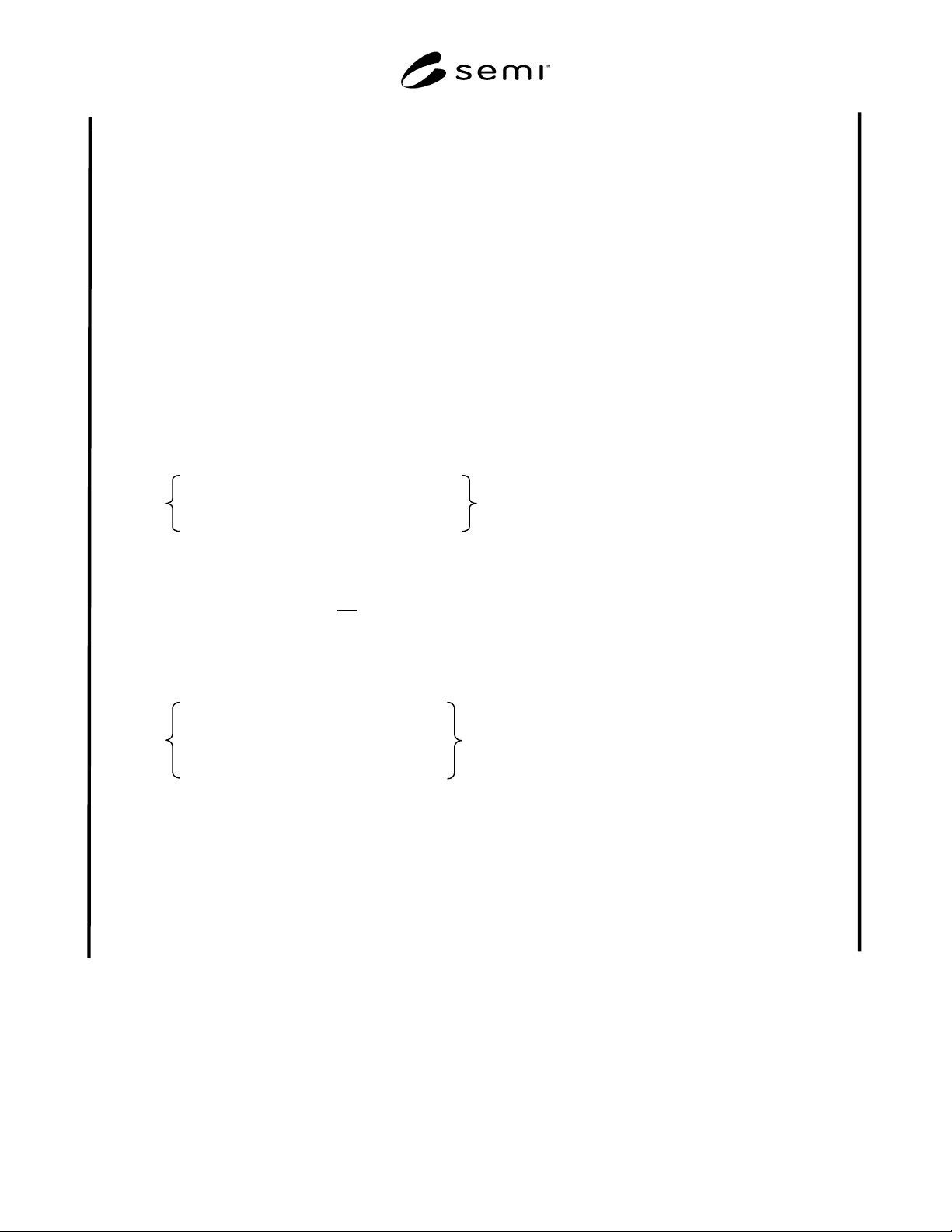
R1-5.7.1 The first time the function is executed, each

module variable is set to zero if the module is in an

unscheduled downtime state and set to one otherwise.

If the function evaluates to 0, the IPF is in an

unscheduled downtime state. Each contiguous instance

of process-flow unscheduled downtime is a process-

flow failure. If the function evaluates to 1, the IPF may

be in either a general downtime state or an up state.

i-UD

0, if module i is in an unscheduled down state

1, otherwise

R1-5.7.2 The second time the function is executed,

each module variable is set to zero if the module is in

either a scheduled downtime state OR

an unscheduled

downtime state and set to one otherwise. If the function

evaluates to 0, the IPF is in a general downtime state. If

the function evaluates to 1, the IPF is a neutral state.

i-GD

0, if module i is in scheduled down state

OR an unscheduled down state

1, otherwise

R1-5.7.3 To summarize, if IPF(M

) = 0, the process-

flow state is unscheduled downtime (UD). Otherwise, if

IPF(M

) = 0 the process-flow state is general

downtime (GD), and if IPF(M

) = 1, the IPF state is

uptime.

NOTE 8: The process-flow state for an IPF that has at least

one module in an unscheduled downtime state may be either

(1) unscheduled downtime, (2) general downtime, or (3)

neutral. Condition (1) occurs when the unscheduled downtime

module is serial within the IPF. Condition (2) occurs when the

unscheduled downtime module is not serial within the IPF,

but a module (or set of modules) that is serial within the IPF

is in a scheduled downtime state. Condition (3) occurs when

none of the downtime modules are serial within the IPF

regardless of being in a scheduled or unscheduled state.

R1-6 Determining Multi-Path Cluster Tool

States

R1-6.1 The temporal mapping rules for determining

multi-path cluster tool “productive/unscheduled

downtime/neutral” states from module “productive/not-

productive” states and IPF “up/downtime/unscheduled”

states is as follows:

R1-6.1.1 If any module is in the “productive” state,

then the cluster tool is in the “productive” state.

R1-6.1.2 Otherwise, if all of the IPFs are in the

“unscheduled downtime” state, then the multi-path

cluster tool is in the “unscheduled downtime” state.

R1-6.1.3 Otherwise, the multi-path cluster tool is in the

“neutral” state.

R1-6.2 Each contiguous instance of a multi-path

cluster tool unscheduled downtime state is a multi-path

cluster tool failure.

NOTE 9: This logic is similar to the relationship between

module states and the equipment states in SEMI E116, where

the SEMI E116 “busy” state is analogous to the multi-path

cluster tool “productive state,” the SEMI E116 “blocked”

state is analogous to the “unscheduled downtime” state, and

the SEMI E116 “idle” state is analogous to the “neutral” state.

However, the actual relationship between these two sets of

states is neither trivial, nor direct.

NOTE 10: Productive time may not be easily allocated to

IPFs in the general case. It is expected that some modules will

belong to more than one IPF and that it will be prohibitive to

ascertain the specific flow for each module from moment to

moment. Hence, metrics that depend on productive time may

not be calculated for IPFs.

NOTE 11: For the metrics presented in this document, it is

not necessary to calculate downtime states other than

unscheduled downtime at the multi-path cluster tool level.

The effect of states other than productive and unscheduled

downtime on the multi-path cluster tool is evaluated as the

aggregate effect of such states on the IPFs.

SEMI E10-0304

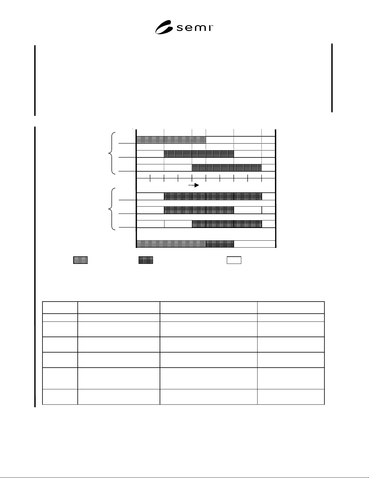
R1-6.3 Example 3 — A simplified example with a

discrete timeline is shown in Figure R1-12. In this

example there are three modules (i.e., M1, M2, M3) and

three IPFs (i.e., IPF1, IPF2, IPF3). IPF1 uses all three

modules, whereas IPF2 does not use M3, and IPF3 does

not use M2. The state value functions for the IPFs are

IPF1 = M1 × M2 × M3, IPF2 = M1 × M2, and IPF3

= M1 × M3, respectively. Temporal mapping of the

IPFs and the multi-path cluster tool is described in

Table R1-4.

NOTE 12: The condition between time t = 4 and t = 5, where

the multi-path cluster tool is productive but all of its IPFs are

down, is expected only as a transient condition in actual

practice. Once the productive module finishes its task in

progress, the multi-path cluster tool would be expected to go

down. However, while the module is productive, it also is

accruing theoretical processing time used in the SEMI E79

metric, rate efficiency. The allocation of this transient

condition to productive time is necessary in order to guarantee

that rate efficiency evaluated over any interval is never

greater than 100%.

100

IPF2

IPF3

IPF1

time

Cluster Tool

Module

EMI E10

States

Process

Flow

Up/Down

States

roductive = Unscheduled Down =

ot-Productive

Figure R1-12

Mapping Cluster-Tool States, Example 3

Table R1-4 Temporal Mapping of Example 3

Time Module Events IPF Events Cluster Tool State

t = 0 M1 is productive. All IPFs are up. Productive

t = 2 M2 goes down.

M1 is still productive.

IPF1 and IPF2 go to unscheduled

downtime.

Productive

t = 4 M3 goes down.

M1 is still productive.

All IPFs are in unscheduled downtime. Productive

t = 5 M1 exits productive state.

No modules are productive.

All IPFs are still in unscheduled downtime. Unscheduled Downtime

t = 7 M2 come back up.

M3 transitions into scheduled

downtime.

IPF2 is up. At least one IPF is up.

IPF1 and IPF3 are down, but not in

unscheduled downtime

Neutral

t = 9 M3 comes back up.

All modules are up.

All IPFs are up. Neutral