semi合集-English.pdf - 第422页
SEMI E56-1104 © SEMI 1996, 2004 11 14.1.1 Accuracy 14.1.1.1 Determine the preci sion at a set point by calculating the standard de viation of al l the measured values (both upscale and downscale) fo r that setpoint. Perf…
SEMI E56-1104 © SEMI 1996, 2004 10
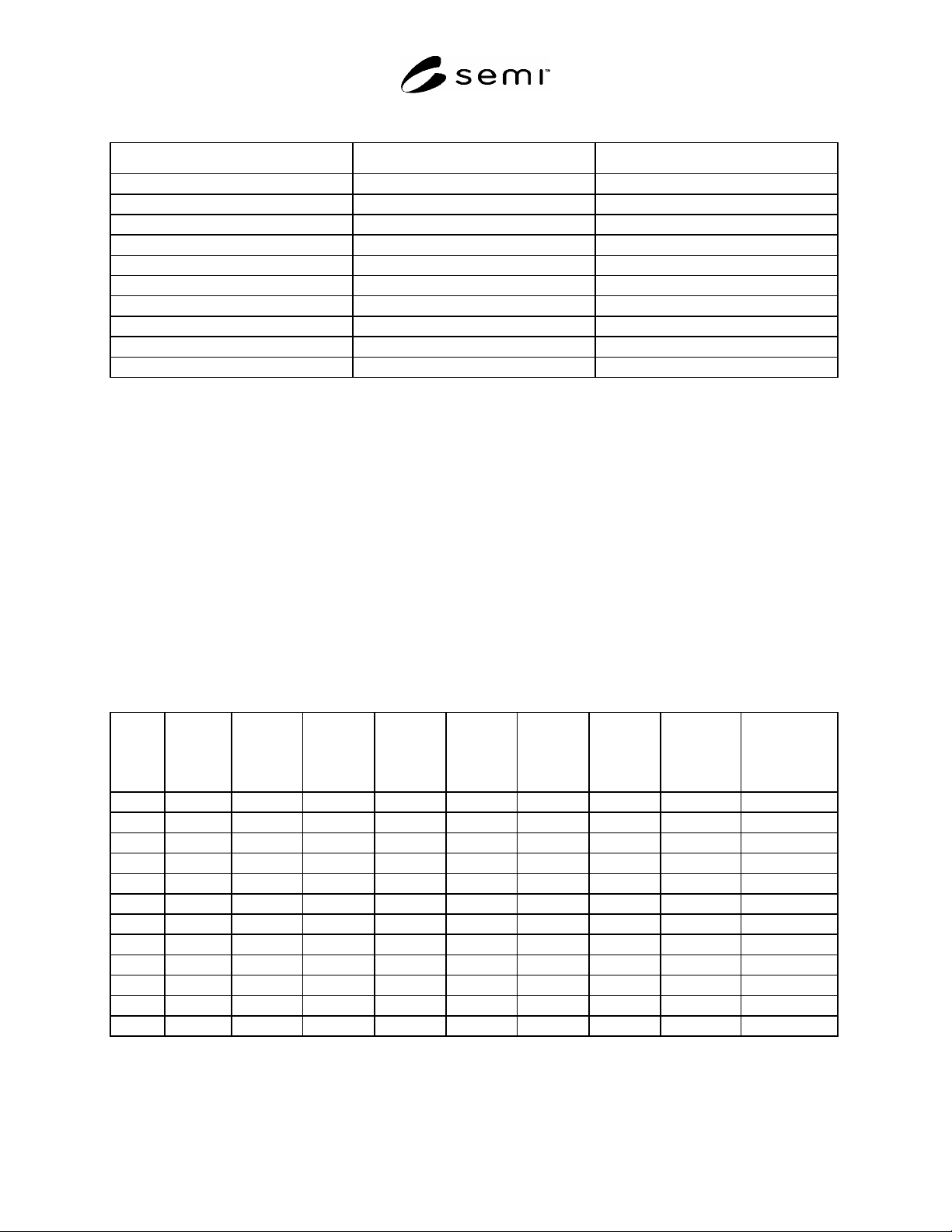
Table 3 Data Tabulation
Setpoint Lower Deadband (sccm) Upper Deadband (sccm)
10%
20%
30%
40%
50%
60%
70%
80%
90%
100%
13.6.2 Step the MFC’s setpoint to the highest setpoint chosen that is less than the upper setpoint limit in the
increments previously chosen; record data at each setpoint.
13.6.3 At each setpoint, slowly increase the setpoint signal to the DUT until a detectable flow output change is
observed in the flow standard.
13.6.4 Record the setpoint signal when the flow output changes and call this the upper deadband value.
13.6.5 Return to the setpoint selected in Section 13.6.3.
13.6.6 Slowly decrease the setpoint signal until a detectable flow output change is observed.
13.6.7 Record the setpoint signal and call it the lower deadband value. Use Table 3.
14 Data Analysis
14.1 Calculations
NOTE 4: NOTE: Record calculations on Table 4.
Table 4 Worksheet for Table 1
Setpoint
Up Ave.
Flow
(sccm)
Down Ave.
Flow
(sccm)
Up/Down
Ave. Flow
(sccm)
Precision
(sccm)
Bias
(sccm)
Accuracy
(%)
Linearity
(%)
Repeatability
Reproducibility
0
10
20
30
40
50
60
70
80
90
100
Over-all

SEMI E56-1104 © SEMI 1996, 2004 11
14.1.1 Accuracy
14.1.1.1 Determine the precision at a setpoint by
calculating the standard deviation of all the measured
values (both upscale and downscale) for that setpoint.
Perform this calculation at each setpoint.
P
(
(
v
i
A
a
)
2
)
j
n
j
P
Precision
v
i
The ith measured value at a setpoint for a given cycle
A
a
Average measured value
n
j
Number of readings at a setpoint at a given cycle
i
Reading number in a cycle for a given setpoint
j
Cycle for a given setpoint
14.1.1.2 Determine the bias at a setpoint by averaging
the difference between the measured value and the sum
of the setpoint and zero offset. Perform this calculation
at each setpoint.
B
=
S – Z)
i
]
j
n
j
B
= Bias
A
= Measured Value
S = Setpoint
Z = Zero offset of DUT
14.1.1.3 Determine the accuracy at each setpoint by
summing the absolute values of the precision and bias.
Divide the sum by the average of the setpoint and
multiply by 100%. The sign of the accuracy is the same
as the sign of the bias. Perform this calculation at each
setpoint.
AS
%
P
B
S
a
100
(
B
B
)
AS
Accuracy of setpoint
S
a
Average of setpoint
14.1.1.4 Determine the overall accuracy of the DUT by
adding the absolute value of the flow standard accuracy
to the maximum absolute accuracy value from Section
14.1.1.3. This value is expressed as ± percentage of
reading.
NOTE 5: This assumes that the flow standard accuracy is
expressed as a percentage of reading.
A
D %
A
S
M
AX
A
D
f
A
D
Accuracy of the DUT
A
D
f
Accuracy of the flow standard
14.1.2 Linearity
14.1.2.1 Determine an equation for the straight line
passing through the indicated flow at zero actual flow
and the average measured value at a 100% setpoint.
m
A
a
Z
a
100
Y
mS
b
Z
a
Indicated flow at zero actual flow
A
a
Average measured value at 100% setpoint
m
Slope
Y
Ideal linearity value
14.1.2.2 Determine the linearity at a setpoint by
averaging the difference between the measured value
and the value of y at a given setpoint. Divide this
number by the full scale range of the DUT and multiply
by 100. Perform this calculation at each setpoint.
Record this value in Figure 7.
L
S%
[
(
A
Y )
i
]
j
F
S
n
j
100
L
S
Linearity of setpoint
F
S
Full scale flow rate
14.1.2.3 The overall linearity of the DUT is the
maximum absolute value calculated in Section 14.1.2.2.
This value is expressed as a ± percentage of full scale.
L
D%
L
S
max
L
D
Linearity of DUT
14.1.3 Repeatability
14.1.3.1 Determine the intermediate value by
calculating the standard deviation of the measured
values for all cycles approaching from a given
direction. Divide this by the average setpoint for these
cycles. Perform this calculation at each setpoint for
both directions. The 100% setpoint will only be
approached from the upscale direction.
I
%
(v
i
A
a
)
2
n
j
S
a
100
I
Intermediate value
14.1.3.2 The repeatability at a setpoint is the
maximum intermediate value at each setpoint calculated
in Section 14.1.3.1. This value is expressed as a ±

SEMI E56-1104 © SEMI 1996, 2004 12
percentage of reading. Perform this calculation at each
setpoint.
RPS
I
max
R
PS
Repeatability at a setpoint
14.1.3.3 The overall repeatability of the DUT is the
maximum value calculated in Section 14.1.3.2.
R
PD
R
P
S
max
R
PD
Repeatability of the DUT
14.1.4 Short-Term Reproducibility
14.1.4.1 Determine the short-term reproducibility at a
setpoint by dividing the precision of the setpoint by the
average setpoint. This is expressed as a percentage of
reading. Perform this calculation a each setpoint.
SRS
P
S
a
100
SRS
Short - term reproducibility at a setpoint
14.1.4.2 The overall short-term reproducibility of the
DUT is the maximum value calculated in Section
14.1.4.1.
SRD
SR
S
max
SRD
Short - term reproducibility of the device
14.1.5 Deadband
14.1.5.1 Determine the absolute deadband value by
subtracting the lower deadband value from the upper
value at each setpoint. Perform this calculation at each
setpoint.
D
D
u
D
l
D
Deadband value
D
u
Upper deadband value
D
l
Lower deadband value
14.1.5.2 Determine the deadband at setpoint by
dividing the absolute deadband value by the initial
setpoint and multiplying by 100. This is expressed as a
percentage of reading. Perform this calculation at each
setpoint.
D
B
S
D
S
100
D
B
S
Deadband of setpoint
14.1.5.3 The overall deadband of the DUT is the
maximum value calculated in Section 14.1.5.2.
D
BD
D
BS
max
D
BD
Deadband of device
14.1.6 Hysteresis
14.1.6.1 Determine the hysteresis plus deadband by
subtracting the average of the difference between the
downscale measured value and the downscale setpoint
from the average of the difference between the upscale
measured value and the upscale setpoint. Perform this
calculation at each setpoint.
H
DB
S
[
(
A
u
S
u
)
i
]
k
n
k
[
(
A
l
S
l
)
i
]
n
n
m
H
DB
S
Hysteresis plus deadband at a setpoint
A
u
Measured value, up cycle
A
l
Measured value, down cycle
S
u
Setpoint, up cycle
S
l
Setpoint, down cycle
n
N
umber of up scale readings
k
Up cycle number for a given setpoint
m
Down cycle number for a setpoint
14.1.6.2 Determine the hysteresis by subtracting the
deadband from hysteresis plus deadband and divide the
result by the initial setpoint and multiply by 100. This
is expressed as a percentage of reading. Perform this
calculation at each setpoint.
H
S
H
DBS
D
S
100
H
S
Hysteresis at a setpoint
14.1.6.3 The overall hysteresis of the DUT is the
maximum value calculated in Section 14.1.6.2.
H
D%
H
S
max
H
D
Hysteresis of dev
i
15 Data Presentation
15.1 Accuracy — Plot the accuracy data at each
setpoint on a graph. The x-axis is the setpoint, and the
y-axis is accuracy as a percentage of the reading.
15.2 Linearity — Plot the linearity at each setpoint on a
graph. The x-axis is the setpoint, and the y-axis is
linearity as a percentage of full scale.