semi合集-English.pdf - 第5813页
SEMI P24-94 © SEMI 1994, 2004 4 8 Related Documents “ASTM Com pilation of ASTM Standard Defi nitions,” American Society for Testi ng and Materials, 100 Barr Harbor Drive, West Conshohoken, P A 19428. Nyyssonen, Dr. Rober…

SEMI P24-94 © SEMI 1994, 2004 3
6 Procedures to Benchmark Precision
6.1 Precision Types
6.1.1 Static Precision — A series of measurements
made of a single feature where, for each measurement,
the information is reacquired and reprocessed. The
minimal intervention required to repeat the
measurement will be used. The standard deviation will
be calculated based on the sample data.
6.1.2 Z (Axis Adjustment) Precision — A series of
measurements is made of a single feature where it is
necessary to refocus before each measurement (without
intentional movement in the x and y axes before each
measurement). The standard deviation will be
calculated based on the sample data.
6.1.2.1 Dynamic Precision — Make one measurement
of grouped line and space features at n number of sites
on a focus/exposure matrix wafer, which includes
typical size and side wall angle variations. Remove the
wafer from the system, then reload and remeasure.
Compute the dynamic precision, 3s, by the double
sample method (see Section 8.1.3).
6.1.2.1.1 A total of 1 size × n sites × 2 repeates = 2n
measure-ments per wafer × 3 passes = 6n
measurements required.
6.1.2.1.2 10 is a minimum recommended value for n.
6.1.2.1.3 This may also be redone for different
thicknesses of lines to be measured and repeated for
each of the wafer types in the process.
7 Precision Test
7.1 Test Methods
7.1.1 Stability Test Method — Makes a group of five
measurements of a stable feature, such as etched
polysilicon, at the same position, daily. Any system
adjustment, maintenance, environment variation is
allowed, but noted. Recalibration is optional, but is
noted. Use a feature which doesn’t change over time,
or with repeated measurements. Plot the daily averages
on an individual control chart with control limits based
on the moving range of the daily averages.
7.1.2 Sequence Test Method — A series or sequence of
measurements is taken of the same physical location.
Any change between measurements determines the type
of precision tested.
7.1.3 Double Sample Test Method — Two
measurements are taken at separate times within the test
run at a number of different physical locations. A
series of sites is used which have: same nominal size,
same proximity of other features, similar side wall
angle, etc.
7.2 Test Duration
7.2.1 Short Term — No system calibration, adjustment,
or maintenance will be done. The period should be
short enough to minimize the effect of environmental
variations. See R1-1.
7.2.2 Long Term — Any system adjustments,
maintenance, environment variation is allowed. See
R1-2. Recalibration is optional.
7.2.3 Presentation of Results — Some information,
relative to the data, must be included to qualify the
results. Graphical representation of the data is
recommended.
7.2.3.1 The following must be included:
The estimated (1, 2, or 3) standard deviation(s),
Short or Long Term
Confidence interval (see Application Note A.3)
The number of measurements or sample size (n)
Describe the feature film and substrate film
Nominal or average measurement
Feature Type: line or space or hole, grouped or
isolated
The frequency of recalibration
Test identified as the type performed
7.2.3.1.1 Additional information which should also be
included, particularly with unusual conditions, are:
Metric units are recommended, such as nanometer
[nm] or micrometer [µm]
Feature characteristics, such as: sidewall angle,
wall profile, corner radius, materials, thickness,
index of refraction, edge waviness, edge roughness
Duration of the test
The sample frequency
Significant parameters such as operator, system
model, serial number, pertinent environmental
conditions, etc.

SEMI P24-94 © SEMI 1994, 2004 4
8 Related Documents
“ASTM Compilation of ASTM Standard Definitions,”
American Society for Testing and Materials, 100 Barr
Harbor Drive, West Conshohoken, PA 19428.
Nyyssonen, Dr. Robert D. Larrabee, “Submicrometer
Linewidth Metrology for the Optical Microscope,” (J.
of Research of National Bureau of Standards, Vol. 92,
No. 3, May/June 1987). National Institute of Standards
and Technology (NIST), Bldg. 202, Room 204,
Gaithersburg, MD 20899.
Dr. Robert D. Larrabee and Dr. Michael T. Postek,
“Precision, Accuracy, Uncertainty and Traceability and
Their Application to Submicrometer Dimensional
Metrology” (Solid-State Electronics, Vol. 36, No 5, pp
673-684, 1993).
SEMASPEC #91090709A-ENG, “Introduction to
Measurement Capabilities Studies,” SEMATECH,
Technology Transfer, 2706 Montopolis Drive, Austin,
TX 78741.
SEMI P24-94 © SEMI 1994, 2004 5
RELATED INFORMATION 1
NOTICE: The material contained in this related information is not an official part of SEMI P24 and is not meant to
modify or supersede the standard in any way. This information is provided as a source of information to aid in the
application of the standard. As such, it is to be considered as reference material only. The standard should be
referred to in all cases. This related information was approved for publication by full balloted procedures.
R1-1 Short Term Test Duration
R1-1.1 It is recommended the short term test duration
be 30 measurements done in the shortest possible time
under the most limited of conditions to eliminate
extraneous sources of variation.
R1-2 Long Term Duration
R1-2.1 Common practice requires about 30 degrees of
freedom in the highest level of sources of variation.
For example, one should continue a long term study
over 30 working days, if days is the highest level of
variation.
R1-3 Confidence Interval
R1-3.1 This is one way in which confidence interval is
calculated.
vs
2
x
v
.1
/2
2
2
vs
2
x
v
.
/2
2
where
v = df in the extimated standard deviation,
/2 – the alpha risk accepted for the estimate (1-) is
the “confidence level”, and
X
2
refers to the “chi-square” distribution which fits
variances. The equation is arranged such that the area
under the chi-square distribution is to the right of the
designated value.
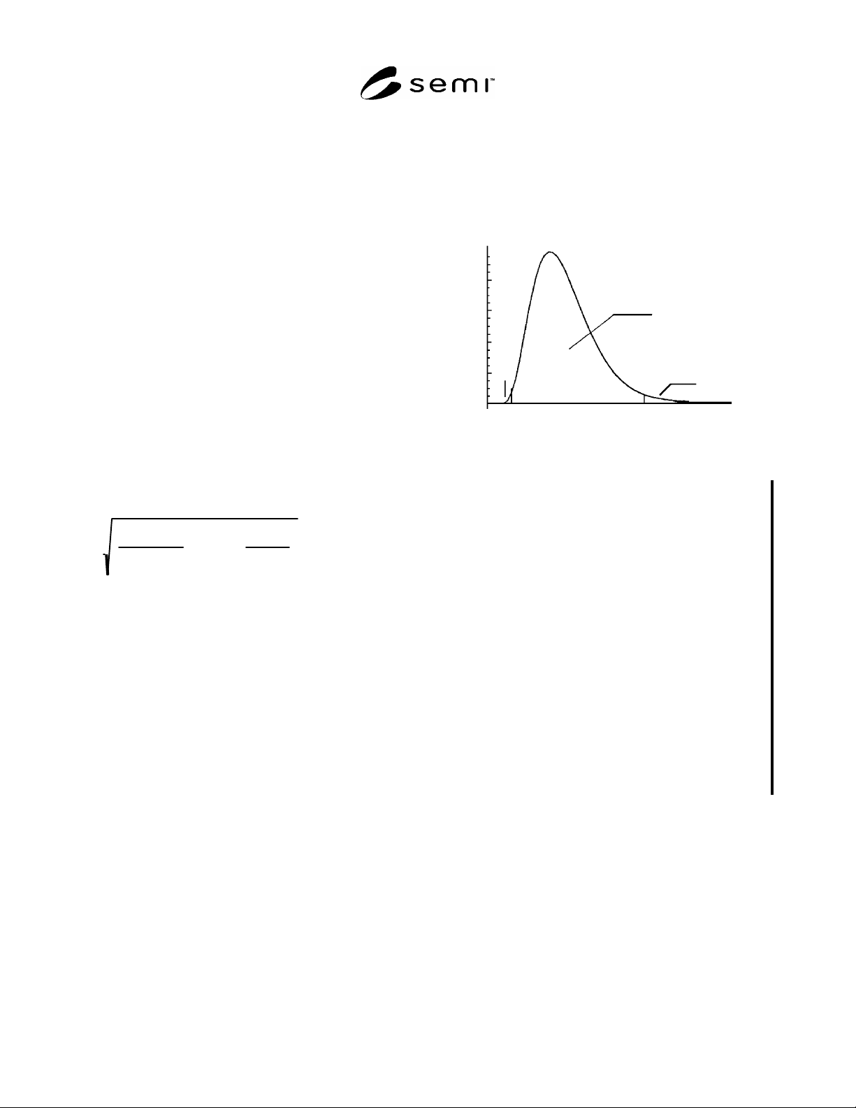
R1-3.2 The reference distribution looks something like
Figure R1-1 — its shape depends on the degrees of
freedom in the estimate.
0
1-
/2
/2
Figure R1-1
Example of a Chi-Square Distribution
NOTICE: SEMI makes no warranties or
representations as to the suitability of the standards set
forth herein for any particular application. The
determination of the suitability of the standard is solely
the responsibility of the user. Users are cautioned to
refer to manufacturer's instructions, product labels,
product data sheets, and other relevant literature,
respecting any materials or equipment mentioned
herein. These standards are subject to change without
notice.
By publication of this standard, Semiconductor
Equipment and Materials International (SEMI) takes no
position respecting the validity of any patent rights or
copyrights asserted in connection with any items
mentioned in this standard. Users of this standard are
expressly advised that determination of any such patent
rights or copyrights, and the risk of infringement of
such rights are entirely their own responsibility.
Copyright by SEMI® (Semiconductor Equipment and Materials
International), 3081 Zanker Road, San Jose, CA 95134. Reproduction of
the contents in whole or in part is forbidden without express written
consent of SEMI.