semi合集-English.pdf - 第7565页
SEMI MF1811-0704 © SEMI 2003, 2004 12 5.3 RMS Slope 5.3.1 There are two dif fer en t estimators for the rms slope, ∆ q — one expressed in configuration space, and the other in freque ncy space, as follows: ∑ − = − + = ∆ …

SEMI MF1811-0704 © SEMI 2003, 2004 11
where M
0
(and also M
1
and M
2
) are evaluated using the
general moment expression,
∑
=
=
N
n
P
P
nZn
N
M
1
)(
1
(23)
where:
P = 0, 1, or 2.
5.1.3 Piston and tilt detrending is as follows:
][)()( nbanZndZ
)
)
)
+−= (24)
where:
n = 1, 2, … , N,
a
)
=
]3)12[(
1
2
10
MMN
N
−+⋅
−
+ , and
b
)
=
+
−
−
−
1
2
1
6
1
0
N
M
M
N
.
5.1.4 Piston, tilt, and curvature detrending is as
follows:
][)()(
2
ncnbanZndZ
)
)
)
)
++−= (25)
where:
n = 1, 2, … , N,
a
)
=
],10)12(6)233[(
)2)(1(
3
210
2
MMNMNN
NN
++−++
−−
+
b
)
=
and],)1(30)118)(12(2
)12)(2)(13[(
)4)(1(
6
21
0
22
MNMNN
MNNN
NN
++++−
+++
−−
−
c
)
=
.6)1(6)2)(1[(
)4)(1(
30
210
22
MMNMNN
NN
++−++
−−
+
NOTE 1: The estimated values of the coefficients depend on
the degree of the polynomial being detrended. For example,
the value of the coefficient a
)
for piston detrending and
piston-plus-tilt detrending derived from the same data set are
generally different.
NOTE 2: Despite these apparent differences, the mean values
of each of the detrended profiles given by
∑
=
==
N
n
ndZ
N
1
0)(
1
Mean value
)
(26)
vanishes in all cases. This means that the “dc” value of the
estimated power spectrum of the detrended profile is zero,
which offers a convenient numerical check on the numerical
processing routines used.
NOTE 3: Least-squares fitting routines are available in many
computer packages. Analytic results are given above for
reference and checking.
5.2 RMS Roughness
5.2.1 There are two different estimators for the rms
roughness, R
q
— one expressed in configuration space,
and the other in frequency space, as follows:
∑
=
=
N
n
q
ndZ
N
R
1
22
)(
1
)Config(
))
(27)
and
∑
+
=
=
2
1
1
1
2
)(
1
)Freq(
N
m
q
mS
ND
R
)
)
(28)
1 where )(
1
mS
)
is the periodogram estimate of the PSD
based on )(ndZ
)
(see Section 5.4).
NOTE 4: These two estimates of R
q
2
are mathematically
identical if the periodogram is evaluated using a unit data
window, W(n) = 1. Although a unit window function is not
recommended for general use, the numerical identity of the
Equation 27 and Equation 28 in that case offers a convenient
check on the programming of the periodogram estimator.
NOTE 5: If a non-unit data window is used in the calculation
of the PSD the two estimates of the rms roughness given will
not, in general, be numerically identical for a particular pro-
file measurement. On the other hand, the two estimates are
identical for an ensemble average over a large number of pro-
file measurements. In other words, the two estimates of R
q
2
are statistically the same.
NOTE 6: The first estimator has the advantage of familiarity
and simplicity since it is expressed directly in terms of the
detrended values of the measured profile data. Its disad-
vantage is that it involves, perforce, the transfer function of
the measuring apparatus, and in a nonobvious way. In con-
trast, the frequency-space form may be more complicated to
evaluate but has the advantage that it permits the bandwidth to
be included in the rms value to be varied by selecting the
range of m values included in the frequency sum. In addition,
it permits the effects of a non-unit instrumental transfer
function within that bandpass to be examined directly, and to
be divided out by restoration processes, if its form is known
independently.
NOTE 7: The spectra of real surfaces frequently tend to
diverge at low spatial frequencies so that the values of the rms
roughness obtained using either estimator may depend signi-
ficantly on the value of the LFL of the measurement process,
or chosen as a reference value. In some cases, the presence of
a non-vanishing LFL can give a finite value of the profile
roughness when its intrinsic value is infinite or undefined.
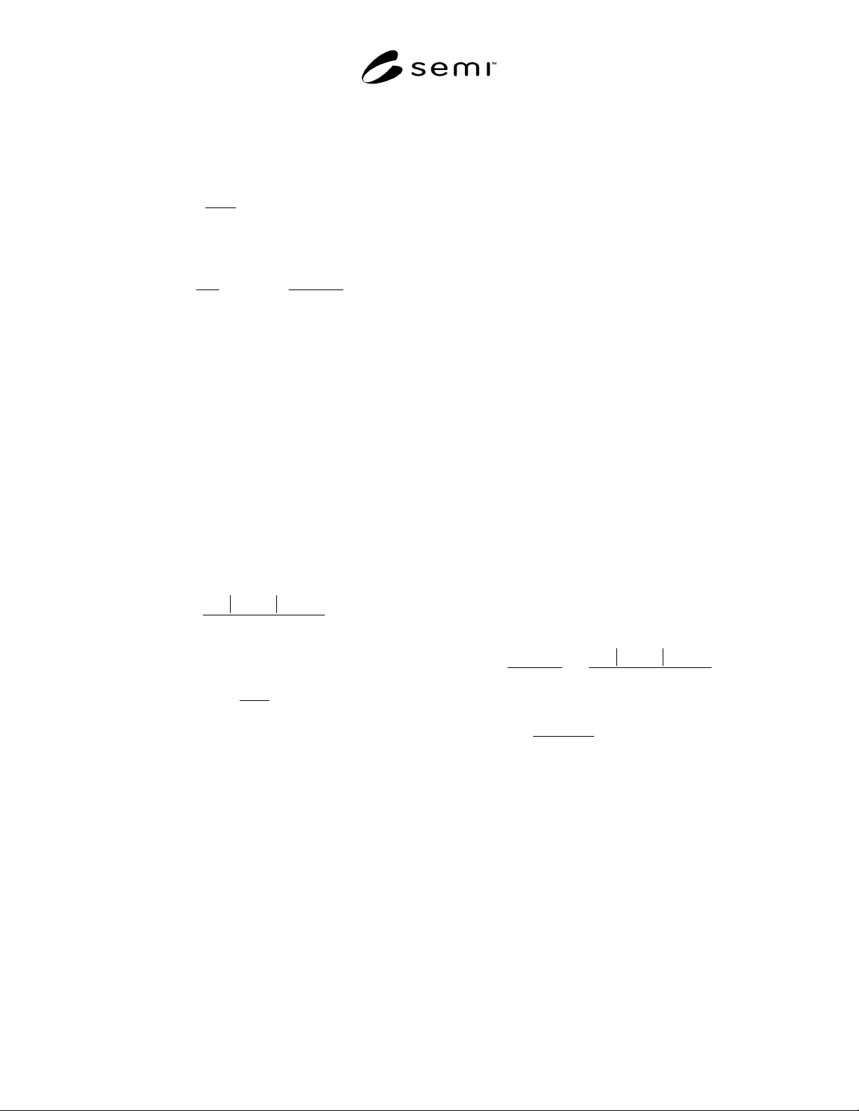
SEMI MF1811-0704 © SEMI 2003, 2004 12
5.3 RMS Slope
5.3.1 There are two different estimators for the rms
slope, ∆
q
— one expressed in configuration space, and
the other in frequency space, as follows:
∑
−
=
−+=∆
1
1
2
2
)()1([
1
)Config(
N
n
q
ndZndZ
ND
)))
(29)
and
2
)2/(1
1
1
2
)1(2
)(
1
)Freq(
−π
=∆
∑
+
=
ND
m
mS
ND
N
m
q
)
)
(30)
NOTE 8: The magnitudes of these two estimates are
generally different since the first treats the profile as a
collection of straight-line segments connecting the
measurement points, while the second connects them with a
bandwidth-limited interpolation curve and involves a smaller
bias error.
NOTE 9: The notes for the rms roughness estimators just
made generally apply to slope estimates as well. One
difference is that the significant bandwidth effects on the
slope occur principally at the HFL rather than the LFL as is
the case for rms roughness measurements.
5.4 Periodogram Estimators of the Profile Power
Spectral Density
5.4.1 Form for 1-dimensional Power Spectral Density
for height-measuring profilometers is as follows:
.
)()(FFT2
)(
2
1
N
mKmD
mS
⋅⋅
=
)
(31)
The spatial frequency is evaluated at the discrete
valuesof m, with m = 1, 2, … , [1 + (N/2)]:
.
1
ND
m
f
x
−
= (32)
5.4.2 The symbol FFT in Equation 31 stands for
discrete Fourier transform, which is always evaluated
using some version of the fast Fourier transform as
follows:
∑
=
⋅⋅−−π=
N
n
ndZnWNmnim
1
)()(]/)1)(1(2exp[)(FFT
)
(33)
where:
W(n) = window function (see Section 5.6) and
K(m) = book-keeping factor equal to ½ for m = 1 o
r
m = 1 + (N/2) and equal to 1 otherwise.
NOTE 10: Equation 33 applies for the conventional case of
even N. Different forms apply for odd N.
NOTE 11: The case m = 1 corresponds to the zero-frequency
or dc component of the detrended surface profile and m = 2
corresponds to the spatial frequency 1/(ND), which is
essentially the reciprocal of the trace length, ( N–1)D. On the
opposite extreme, the frequency corresponding to m = 1 + N/2
is the Nyquist frequency, 1/(2D). The extreme range of
surface wavelengths included in the measurement is therefore
1/(ND) < f < 1/(2D). In other words, the extreme LFL =
1/(ND), the extreme HFL = 1/(2D), and the dynamic range of
the measurement is N/2.
NOTE 12: A convenient and readable reference to the FFT
and its evaluation is Chapter 12 in Numerical Recipes by
Press, Flannery, Teukolsky, and Vetterling (see Section 7.1).
NOTE 13: The Brookhaven National Laboratory Report (see
Section 7.2) contains further background information on these
procedures along with a computer program and numerical
examples. (The BASIC routines used there involve different
forms for the quantities M
P
appearing in the expressions for
the detrending polynomials than those discussed in this guide,
although the numerical values of the detrending polynomials
are identical in both cases.)
NOTE 14: The periodogram estimator just given is not the
only method of estimating the power spectral density from a
set of profile data, but it is the most direct and common
method. It is sufficient for general use, and is a necessary
first step to be taken before adding embellishments such as
post-processing or considering more complicated estimators.
This guide does not exclude the use of post-processing or
alternative methods of analysis, but does require that the basic
periodogram estimates just described be included in the
discussion for comparative purposes.
5.4.3 Form for 1-dimensional Power Spectral Density
for slope-measuring profilometers is as follows:
N
mKmD
ND
m
mS
)()(FFT2
)1(2
)(
2
2
1
⋅⋅
⋅
−π
=
−
)
(34)
where:
∑
=
−−π
⋅⋅=
′
N
n
N
mni
ndMnWem
1
)1)(1(2
)()()(TFF
)
and )(ndM
)
is the value of the profile slope measure-
ments detrended using either the least-squares piston or
the piston-plus-tilt expressions (see Section 5.1).
NOTE 15: This estimate of the profile power spectrum is the
power spectrum of the profile slope divided by (2πf
m
)
2
. The
prime on the FFT on the left denotes that it involves slope
rather than height data.
NOTE 16: The case m = 1 corresponds to zero spatial fre-
quency and must be excluded in the use of the above
expressions.

SEMI MF1811-0704 © SEMI 2003, 2004 13
5.5 Periodogram Estimators of the Rms Profile
Roughness and Slope
5.5.1 The periodogram estimator of the rms profile
height, ,
q
R
)
is as follows:
∑
+
=
=
)2/(1
2
1
)(
1
N
m
q
mS
ND
R
)
)
(35)
This quantity has the same dimension as the original
height measurements and is independent of the
magnitude and dimensions of the sampling interval, D.
5.5.2 The corresponding estimator for the rms profile
slope, ,
q
∆
)
is as follows:
∑∑
+
=
+
=
−π=
′
=∆
)2/(1
2
1
2
3
)2/(1
2
1
)()1(
)(
1
2)(
1
N
m
N
m
q
mSm
ND
mS
ND
))
)
(36)
In evaluating these quantities the height measurements,
Z, and the sampling interval, D, must be expressed in
the same length units. Although
q
∆
)
is in units of
radians, its magnitude scales as 1/D.
5.6 Window Functions
5.6.1 Window functions appear in a wide variety of
signal-processing applications, with different shapes
and normalizations. Although this guide recommends
the use of the Hann or Blackman window, other forms
are included for comparison. All are normalized so that
∑
=
=
N
n
nW
N
1
2
1)(
1
in order to preserve the magnitudes of
average values of the mean-square profile statistics.
5.6.2 Particular forms are:
5.6.2.1 Rectangular or Daniell window:
1)( =nW (37)
5.6.2.2 Hann, or Raised Cosine window:
−π
−=
N
n
nW
)1(2
cos124
1728
2
)(
(38)
5.6.2.3 Hamming window:
−π
−⋅=
N
n
nW
)1(2
cos2327
1987
2
)(
(39)
5.6.2.4 Blackman window:
−π
+
−π
−⋅=
N
n
N
n
nW
)1(4
cos4
)1(2
cos2521
1523
2
)(
(40)
NOTE 17: The choice of window functions is of minor
importance for randomly-rough surfaces as long as it
smoothes the data at the ends of the data record. The
rectangular or Daniell window does not do this, but is useful
for numerical checking.
NOTE 18: In the case of profiles with a smooth PSD, the
principal effect the window shape is to change the fine-scale
fluctuations in the periodogram estimate without changing its
ensemble-average value, except, perhaps, near the LFL.
NOTE 19: In the case of profiles involving periodicities, the
window shape can change the shape of the sharp lines in the
PSD, albeit without changing their areas. The choice of the
window shape then involves a trade-off between line width
and smoothness. The raised Hann or Blackman windows are
recommended for general use.
NOTE 20: If the estimation routines are applied to
deterministic profiles, such as individual steps, pits, or bumps,
a data window must still be used to minimize effects of the
finite data record, but the object should be placed in the center
of the profile where the window function is relatively flat.
5.7 Zero Padding
5.7.1 The fastest FFT routines require the total number
of data points to be a power of two, such as N = 2
10
=
1024. If the number of measured points, N, is not a
power of two but lies between 2
a
and 2
b
, the power-of-
two routines can be used by dropping N−2
a
points from
one end of the original data set, or by adding 2
b
−N
zeros and replacing N in the routines everywhere by 2
b
.
5.7.2 The first method is wasteful of data, while the
second uses the full set of measured data but requires
that the estimated PSD be renormalized by multiplying
it by the factor 2
b
/N.
5.8 Averaging of Statistical Quantities:
5.8.1 Power spectral density functions, the mean-
square roughness, and slope values estimated from a
number of individual profiles that have the same
statistical properties can each be averaged together to
obtain composite results. In the case of homogeneously
and isotropically rough surfaces the profiles can lie in
any position and direction on the surface under test. In
the case of homogeneously but anisotropically rough
surfaces they can lie anywhere on the surface but must
lie parallel with each other, preferably perpendicular to
the surface axis. Averaging data lowers the errors
associated with individual measurements.
6 Numerical Test Sequences
6.1 Table 1 presents a set of numerical data for testing
the execution of the users’ implementations of
algorithms discussed in Section 5.
6.2 Although these simulated profile data are in
standard notation, they have been generated by a