semi合集-English.pdf - 第955页
SEMI E124-1103 © SEMI 2003 10 R1-1.5 Now suppose th e factory is managed with a pull strategy where a c onstant WIP level is e nforced so that throughput rates are allowed to reach their equilibrium state. In general, th…
SEMI E124-1103 © SEMI 2003 9
critical WIP
(W
0
= R
max
×T
min
)
Worst Case (throughput-rate & cycle-time efficiency =1/W
0
)
T
min
1
Best Case (throughput-rate
& cycle-time efficiency = 1)
actual
throughput rate
1/T
min
bottle-
neck
through-
put rate
(R
max
)
1
Threshold Case (normalized
production efficiency = ½)
WIP capacity
(W
max
)
average WIP
Green
Yellow
Red
Figure R1-2
Plot of Actual Throughput Rate vs. Average WIP
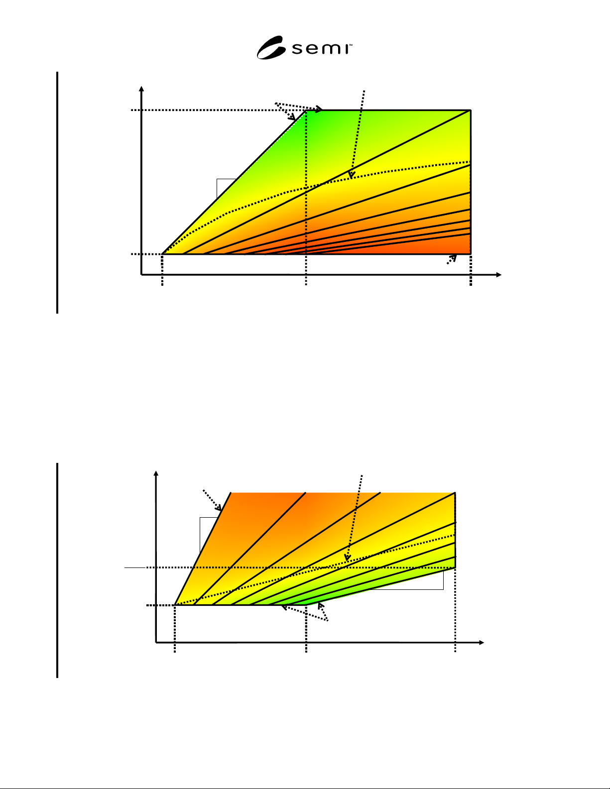
R1-1.3 If we look at two of these fundamental quantities at a time, the factory dynamics become more clear. For
example, Figure R1-2 above shows actual throughput rate as a function of average WIP levels. Here the diagonal
solid black lines represent different constant cycle times, but no known strategy will keep the factory operating
exactly on one of these lines.
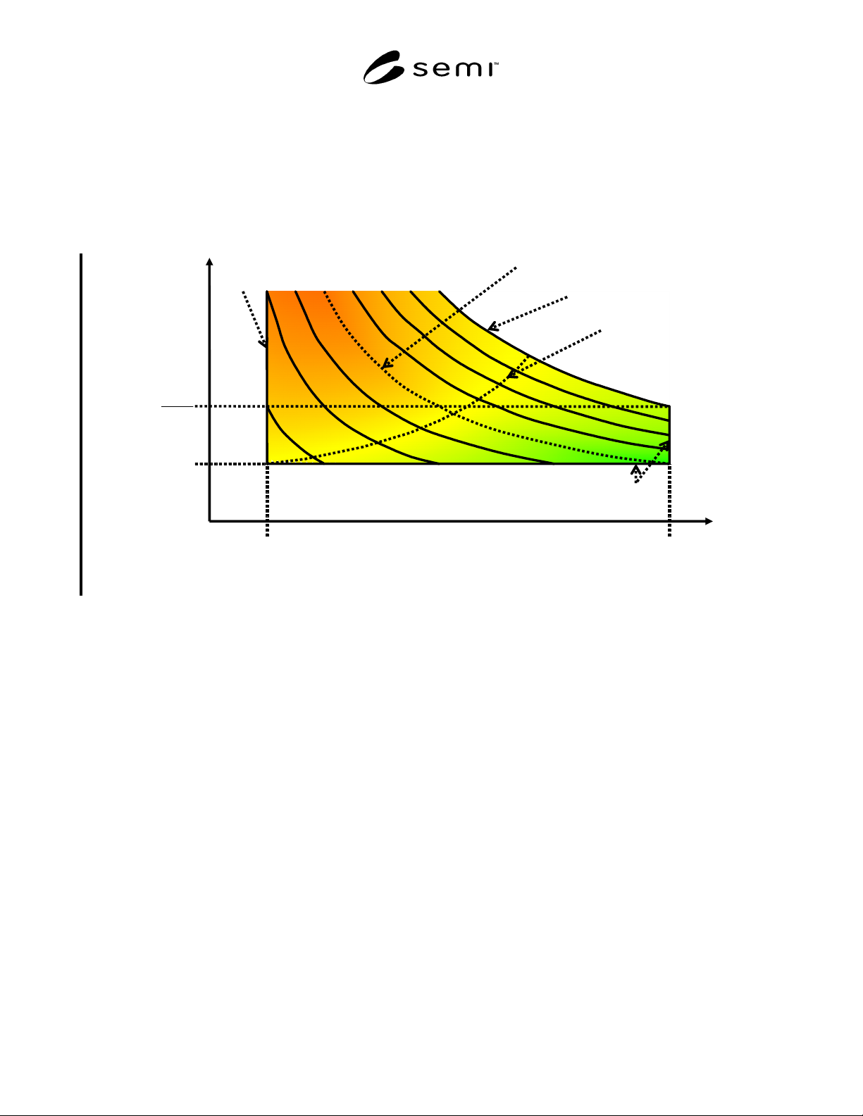
R1-1.4 Now suppose the factory is managed with a push strategy where a constant throughput rate is enforced so
that WIP levels are allowed to reach their equilibrium state. As shown below in Figure R1-3, this amounts to
choosing to operate the factory on one of the diagonal solid black lines (each of which represent different constant
throughput rates). We try to drive the factory along that line toward the bottom left (for lower average cycle time
and average WIP levels) by using better operating principles, but we are resisted by the inherent variability of the
factory.
average
cycle time
theo-
retical
cycle
time
(T
min
)
average WIP
1
bottleneck throughput
rate (R
max
)
Threshold Case (normalized
production efficiency = ½)
critical WIP
(W
0
= R
max
×T
min
)
WIP capacity
(W
max
)
Worst Case (throughput-rate
& cycle-time efficiency = 1/W
0
)
T
min
1
1
Best Case (throughput-rate
& cycle-time efficiency = 1)
W
max
R
max
G
r
e
e
n
Y
e
l
l
o
w
Red
Figure R1-3
Plot of Average Cycle Time vs. Average WIP
SEMI E124-1103 © SEMI 2003 10
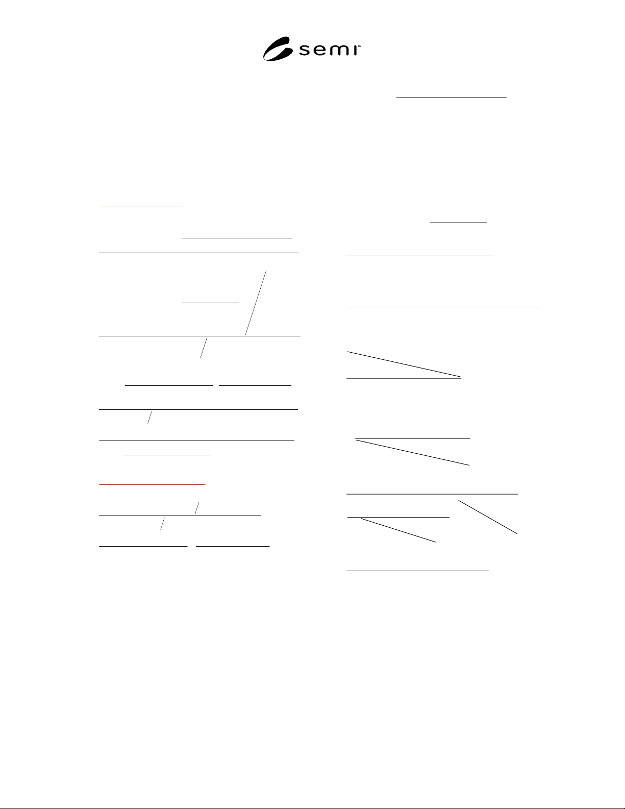
R1-1.5 Now suppose the factory is managed with a
pull strategy where a constant WIP level is enforced so
that throughput rates are allowed to reach their
equilibrium state. In general, this is a better strategy,
because studies have shown that a constant WIP level
will result in a higher average throughput rate than the
constant throughput rate that results in the same average
WIP level. As shown below in Figure R1-4, this
constant WIP strategy (known as CONWIP) amounts to
choosing to operate the factory on one of the solid black
curves (each of which represents a different constant
WIP level). We try to drive the factory along that curve
toward the bottom right (for lower average cycle time
and a higher actual throughput rate) by using better
operating principles, but we are resisted by the inherent
variability of the factory.
actual throughput rate
1/T
min
bottleneck
throughput
rate (R
max
)
Threshold Case
(normalized
production
efficiency = ½)
critical WIP (W
0
= R
max
×T
min
)
WIP capacity (W
max
)
Best Case (throughput-rate & cycle-time efficiency = 1)
average
cycle time
theo-
retical
cycle
time
(T
min
)
W
max
R
max
Worst Case (throughput-rate
& cycle-time efficiency = 1/W
0
)
G
r
e
e
n
Yellow
Red
Figure R1-4
Plot of Average Cycle Time vs. Actual Throughput Rate
SEMI E124-1103 © SEMI 2003 11
R1-1.6 We can now see why the efficiency of
throughput rate and cycle time can both be measured by
the same metric (throughput-rate and cycle-time
efficiency). The following derivation also gives
alternative definitions for throughput-rate and cycle-
time efficiency for use when cycle time information is
not available (such as in resource-based simulations).
(
)
-
-
throughput rate and
cycle time efficiency
()
()
()
max ,
max ,
-
average WIP
theoretical
cycle time
bottleneck throughput rate
average cycle time
average
WIP
theoretical
cycle ti
best case cycle time
average cycle
me
bottleneck
throughput
rat
time
e
=
=
=
()
()()
()
()
1
max ,
1
min
average
WIP
average average
cycle time WIP
theoretical cycle time
bottleneck
average WIP
throughput rate
actual throughput rate
actual throughput rate
average WIP
theoretical cycle
=
=
()
()()
()( )
,
-
bottleneck
throughput rate
time
finished units out total time
average WIP theoretical cycle time
act
theoretical cycle time finished units out
ual throughput
total ti
rate
best case throughput rat
m
e
ea
=
=
=×
()()
as a fraction of
verage WIP
theoretical cycle time WIP
total time turnover
=×
(2)
R1-1.7 The production efficiency is normalized by the
power of the normalizing exponent so that a value of ½
for the normalized production efficiency indicates that
the factory is performing at the level of the threshold
case (which divides a well run factory from one badly
operated). This threshold case is also known as the
practical worst case, because it represents what the best
operating procedures can do in a maximally random
factory (see the Factory Physics book for more on this
case). In the threshold case,
()
(
)
(
)
1
average critical
WIP WIP
average
cycle time
bottleneck throughput rate
+−
= (3)
which results in the following production efficiency.
(
)
production
efficiency
(
)
(
)
()
()
()
()
-
-
max ,
max
throughput rate and WIP
cycle time efficiency efficiency
average
WIP
theoretical
cycle time
bottleneck
throughput
rate
WIP
efficiency
average cycle time
bo
theoretical
cycle time
=×
=×
×
=
()
()( )
()
()( )
{}
,
max ,
ttleneck
average
throughput
WIP
rate
average bottleneck
cycle time throughput rate
WIP efficiency
critical average
WIP WIP
×
×
=
()( )
{}
()( )
{}
min ,
max ,
average bottleneck
cycle throughput
time rate
critical average
WIP WIP
critical average
WIP WIP
×
×
()( )
{}
()()
()
min ,
1
critical average
WIP WIP
average critical
WIP WIP
bottleneck
throughput rate
=
+−
bottleneck
throughput
rate
×
()()
{}
()()
min ,
1
average critical
WIP WIP
average WIP critical WIP
=
+−
(4)