SG_FSE_SiplaceHF_HF3_00193901-05_eng - 第587页

Edition 09/2005 SIPLACE HF/HF3 Appendix 12 Display text component s Samples scans often ’51 1’ (independent of the scan period setting at ’T ime’) (Closure) T ime is the smallest time unit for re presentat ion of oversho…

SIPLACE HF/HF3 Edition 09/2005

Appendix

– The deviation of position signal of the respective Axes are (without any further action) dis-

played and analysed on the SAT LCD-Display.

The

Positioning time is the ’whole travel time of a positioning’ (Start signal to End signal).

The

Control time is the time from start to the first arrival at the target position.

The

Pull off Time is the time to control the generated overshoots down to limits.

Positioning time = Control time + Pull OFF time

– With ’Return’ <

, ’Oscilloscope-Mode’, and ’Signal line (2 or) 3’ we connect the deviation of

position signal of the respective Axis to the SAT BNC output. We can measure with the free

Osci-input CH2 (CH3) the deviation of position signal synchronous to the other dynamic sig-

nals.

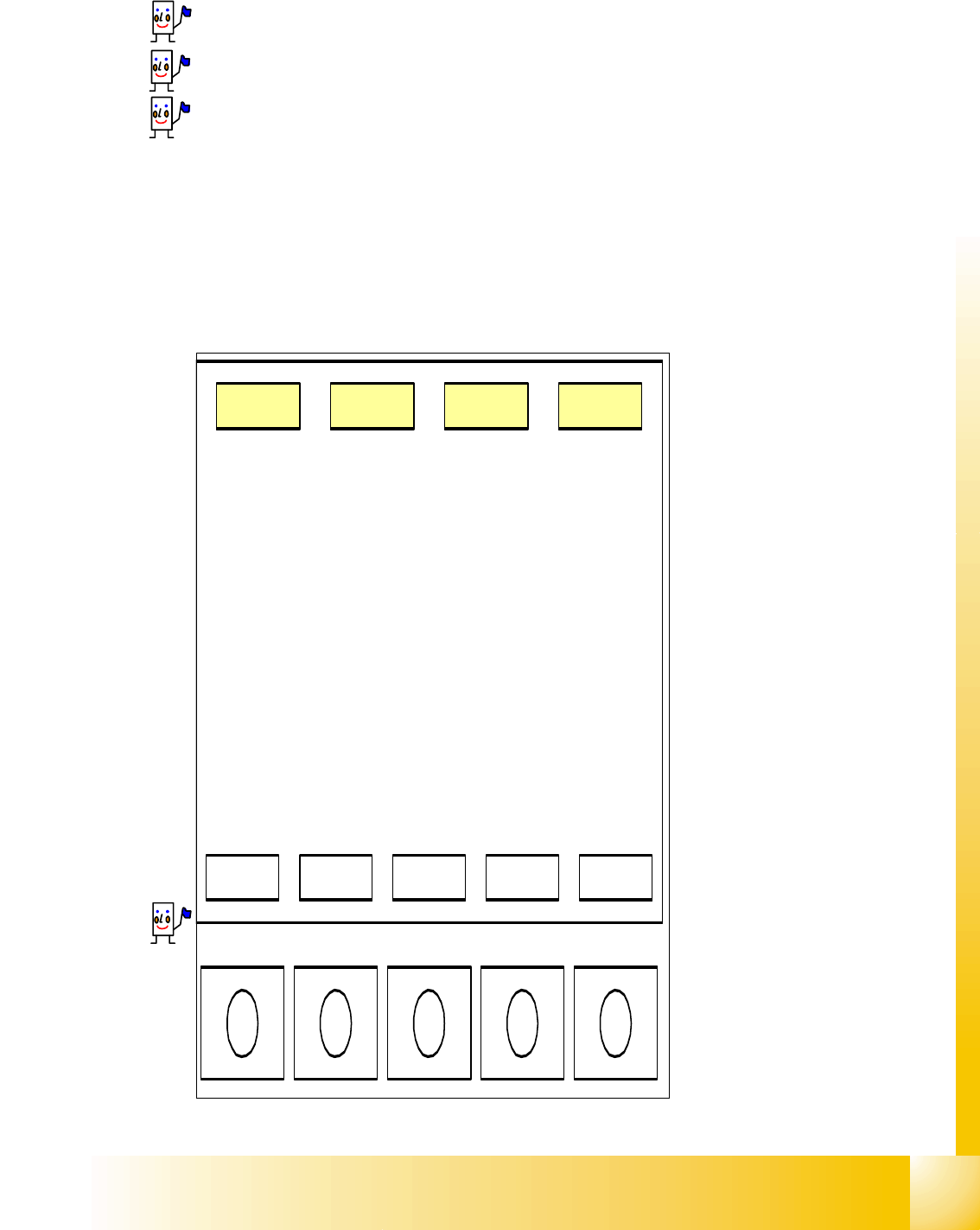
20.3.3.2 SIPLACE Axis Tester ’SAT’ Display

The diagram in the SAT display

shows a typical overshoot (as in

Fig. 20.3 - 7 at the top) and the

corresponding analysis

times.The delays between posi-

tionings should be set long

enough to allow the values to be

read and assessed.

Confirm with <

and select ’PWM

mode’ and ’dynamic’ to display

the position deviation signal on

the oscilloscope. If no overshoot

occurs during the positioning pro-

cess (see Fig. 20.3 - 7 at the bot-

tom) (asymptotic approach), the

positioning time (pos) and the

control time (CTRL) will be

switched simultaneously. There

is therefore no

’pull off time’

(pull off)

during which the over-

shoot is corrected.

PLEASE NOTE:

The display is automatically

scaled to the overshoot size and

time!

Fig. 20.3 - 7 Times and position devia-

tions for a positioning process with/with-

out overshoot

B1 B2 B3 B4 B5

Edition 09/2005 SIPLACE HF/HF3

Appendix

Display text components

Samples

scans often ’511’ (independent of the scan period setting at ’Time’)

(Closure) Time is the smallest time unit for representation of overshoots (scan period) on the dis-

play. Can be reduced with B1 (display is prolonged and details are enlarged) or increased with B2

(display is shortened and whole picture is visible). Adjustment range 0.1 ms to 5 ms.

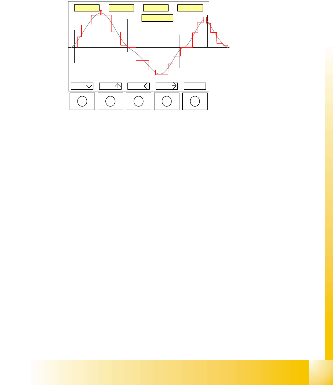
Axis type at the display

(Grain) Scale

is the pixel grouping of a sample (scan period) or digit on the display. 3 / 14 means

that scanning - the time unit entered at Time - will always appear on the screen with a length of 3

(fixed) pixels. A digit position deviation is 14 (dynamic) pixels in this case.

Scope the extent of a maximum positive or negative overshoot

(Time) Range is the signal duration as seen on the screen (alters in line with the ’Time’ setting).

Overshoot!! This is the Position of the axis at the moment of the End signal!

This show you how many Digit has the axis to move after End signal to get really

in target position.

Below the signal you will see a combination of numbers from which one can see at which part

of the overshoot scan the display begins

)

(e.g.

250/511 250th scan overshoot of 511

total scans (pos. 511 = pos.0)

Pull off time is the time measured for the

axis controller to correct the overshoot(s).

Ctrl. Control time is the time needed by

the axis to reach the target position for the

first time. (1)

Pos. Positioning time is the time from axis

start to issuance of the end signal at target

position achievement with reliable position

deviation. Add (1) and (2).

20.3.3.3 Positioning Time Submenus

More specific analyses of the positioning sequence can be performed with the aid of these menus.

After recording a positioning procedure, press <-

Return to open the submenu.

(PWM mode version 1.0) Oscilloscope mode:

The version 1 designation stems from the pulse amplitude modulation used for the representation

of overshoots. It is switched synchronously to the other position deviation signals for the SAT over-

shoot counter, on the oscilloscope.

Start FFT:

The swivel-in process for a particular position can be analyzed with the aid of a frequency spec-

trum. After a positioning procedure, select ’FFT’ (Fast FourierTransformation) to display the

swivel-in spectrum on the screen.

Start Plot:

This menu facilitates measurement of the position deviation signal on the SAT screen, similar to

SIPLACE HF/HF3 Edition 09/2005

Appendix

that performed by the oscilloscope. The full size image is displayed again on the screen and the

operator can scroll with the -> B4 (<- B3) keys. Press <-

Return again to call up a measurement

menu. Mark 1 is at the position of the trigger signal (standard state) but can be displaced with <-

Return, Mark T1 and then B1 or B2. Mark 2 can be positioned at the point to be measured with <-

Return, Mark T2, then B1 and B2.

To print the overshoot control

process for documentation pur-

poses, the signal - as seen on

the screen - can be sent via the

CAN BUS output to a LAPTOP.

The B1/ B2 keys are used to

move the selected mark, while

keys B3/B4 move the image to

the left or right. The ’real’ over-

shoot (gray) is represented in

digital format (red)

20.3.3.4 Overspeed Menu for Assessment of Axis Dynamic

In this menu, the SAT tests the traversing axis for excess nominal speed (maximum speed must

be selected) and shows this positioning procedure as positioning quality. ... Positioning quality ==>

overspeed ==> confirm with <

"Waiting for trigger" ==> SAT waits for ’occurance of overspeed’.

20.3.3.5 System Control

A number of system control submenus could be useful for you, as user, while others should be left

at their default settings.

For example, you should know which menus to use when setting the ’Language’ or ’User level’

(see menu path in following diagram Fig. 20.3 - 8).

The menu point "Save Settings" performs the same backup function as Exit (shutdown proce-

dure).

BNC1 BNC2 BNC3 BNC4

B1 B2 B3 B4 <-

12,25ms

25/317