IPC-TM-650 EN 2022 试验方法--.pdf - 第393页
z z z z IPC-TM-650 Page 7 of 25 Number 2.5.5.5 Subject Stripline Test for Permittivity and Loss Tangent (Dielectric Constant and Dissipation Factor) at X-Band Date 3/98 Revision C Cartesian screen display shows the S21 p…
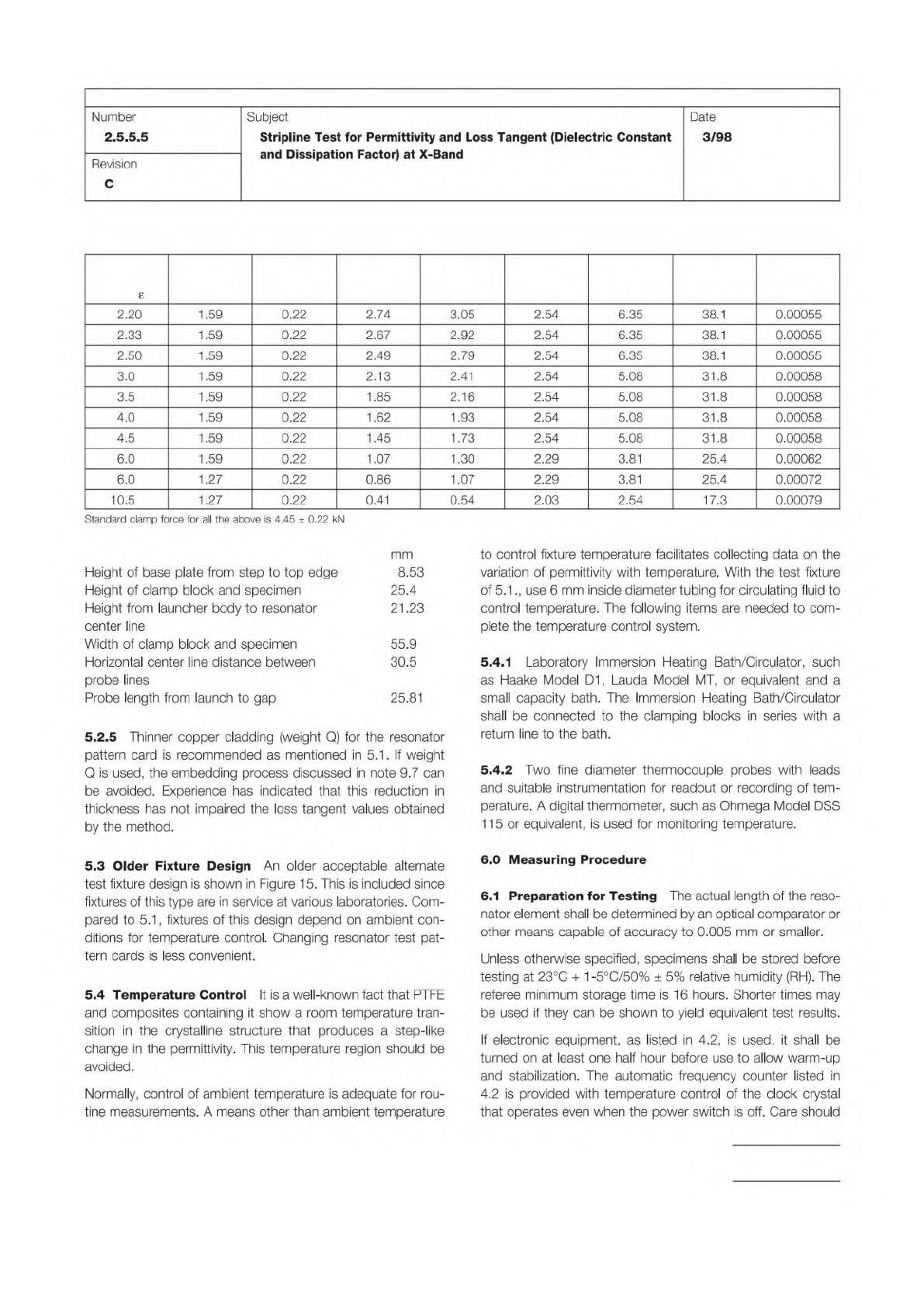
Table 1 Dimensions for Stripline Test Pattern Cards in Millimeters
Nom.
r
Nom.
Thk.
Pattern
Card Thk.
Probe
Width
Chamfer
X, Y
Probe
Gap
Resonator
Width
Resonator
Length 4
Node
1/Q
C
Conductor
Loss
IPC-TM-650
Page 5 of 25
Number
2.5.5.5
Subject
Stripline
Test
for
Permittivity
and
Loss
Tangent
(Dielectric
Constant
and
Dissipation
Factor)
at
X-Band
Date
3/98
Revision
C
Standard
clamp
force
for
all
the
above
is
4.45
±
0.22
kN
£
2.20
1.59
0.22
2.74
3.05
2.54
6.35
38.1
0.00055
2.33
1.59
0.22
2.67
2.92
2.54
6.35
38.1
0.00055
2.50
1.59
0.22
2.49 2.79
2.54
6.35
38.1
0.00055
3.0
1.59
0.22
2.13
2.41
2.54
5.08
31.8
0.00058
3.5
1.59
0.22
1.85
2.16
2.54
5.08
31.8
0.00058
4.0
1.59
0.22
1.62
1.93
2.54
5.08
31.8
0.00058
4.5
1.59
0.22
1.45
1.73
2.54
5.08
31.8
0.00058
6.0
1.59
0.22
1.07
1.30
2.29
3.81
25.4
0.00062
6.0
1.27
0.22
0.86
1.07
2.29
3.81
25.4
0.00072
10.5
1.27
0.22
0.41
0.54
2.03
2.54
17.3
0.00079
mm
Height
of
base
plate
from
step
to
top
edge
8.53
Height
of
clamp
block
and
specimen
25.4
Height
from
launcher
body
to
resonator
21
.23
center
line
Width
of
clamp
block
and
specimen
55.9
Horizontal
center
line
distance
between
30.5
probe
lines
Probe
length
from
launch
to
gap
25.81
5.2
.5
Thinner
copper
cladding
(weight
Q)
for
the
resonator
pattern
card
is
recommended
as
mentioned
in
5.1.
If
weight
Q
is
used,
the
embedding
process
discussed
in
note
9.7
can
be
avoided.
Experience
has
indicated
that
this
reduction
in
thickness
has
not
impaired
the
loss
tangent
values
obtained
by
the
method.
5.3
Older
Fixture
Design
An
older
acceptable
alternate
test
fixture
design
is
shown
in
Figure
15.
This
is
included
since
fixtures
of
this
type
are
in
service
at
various
laboratories.
Com¬
pared
to
5.1
,
fixtures
of
this
design
depend
on
ambient
con¬
ditions
for
temperature
control.
Changing
resonator
test
pat¬
tern
cards
is
less
convenient.
5.4
Temperature
Control
It
is
a
well-known
fact
that
PTFE
and
composites
containing
it
show
a
room
temperature
tran¬
sition
in
the
crystalline
structure
that
produces
a
step-like
change
in
the
permittivity.
This
temperature
region
should
be
avoided.
Normally,
control
of
ambient
temperature
is
adequate
for
rou¬
tine
measurements.
A
means
other
than
ambient
temperature
to
control
fixture
temperature
facilitates
collecting
data
on
the
variation
of
permittivity
with
temperature.
With
the
test
fixture
of
5.1
use
6
mm
inside
diameter
tubing
for
circulating
fluid
to
control
temperature.
The
following
items
are
needed
to
com¬
plete
the
temperature
control
system.
5.4.1
Laboratory
Immersion
Heating
Bath/Circulator,
such
as
Haake
Model
D1
,
Lauda
Model
MT,
or
equivalent
and
a
small
capacity
bath.
The
Immersion
Heating
Bath/Circulator
shall
be
connected
to
the
clamping
blocks
in
series
with
a
return
line
to
the
bath.
5.4.2
Two
fine
diameter
thermocouple
probes
with
leads
and
suitable
instrumentation
for
readout
or
recording
of
tem¬
perature.
A
digital
thermometer,
such
as
Ohmega
Model
DSS
1
15
or
equivalent,
is
used
for
monitoring
temperature.
6.0
Measuring
Procedure
6.1
Preparation
for
Testing
The
actual
length
of
the
reso¬
nator
element
shall
be
determined
by
an
optical
comparator
or
other
means
capable
of
accuracy
to
0.005
mm
or
smaller.
Unless
otherwise
specified,
specimens
shall
be
stored
before
testing
at
23℃
+
1
-5℃/50%
±
5%
relative
humidity
(RH).
The
referee
minimum
storage
time
is
1
6
hours.
Shorter
times
may
be
used
if
they
can
be
shown
to
yield
equivalent
test
results.
If
electronic
equipment,
as
listed
in
4.2,
is
used,
it
shall
be
turned
on
at
least
one
half
hour
before
use
to
allow
warm-up
and
stabilization.
The
automatic
frequency
counter
listed
in
4.2
is
provided
with
temperature
control
of
the
clock
crystal
that
operates
even
when
the
power
switch
is
off.
Care
should
z
z
z
z
IPC-TM-650
Page 7 of 25
Number
2.5.5.5
Subject
Stripline
Test
for
Permittivity
and
Loss
Tangent
(Dielectric
Constant
and
Dissipation
Factor)
at
X-Band
Date
3/98
Revision
C
Cartesian
screen
display
shows
the
S21
parameter
and
the
transmission/incident
power
ratio
in
negative
dB
vertical
scale
units
versus
frequency
on
the
horizontal
scale.
Select
the
start
and
stop
frequency
range
to
sweep
across
the
resonance
peak
and
at
least
3
dB
below
the
peak.
Adjust
the
start
and
stop
frequency
values
as
narrowly
as
possible,
but
still
include
the
resonant
peak
and
the
portions
of
the
response
curve
on
both
sides
of
it
that
extend
downward
3
dB.
6.4.1
The
first
option
is
to
get
the
three
points
(fr,
f1
,
and
f2)
as
described
in
6.2
and
6.3.
Determine
the
resonant
dBr
and
frequency
fr
values
for
the
highest
point
(maximum)
on
the
response
curve.
With
manual
operation,
instrument
program
features
are
available
to
do
this
very
quickly.
On
the
response
curve
to
the
left
and
right
of
fr,
locate
the
,
dB〕
and
f2,
dB2
points
as
near
as
possible
to
3
dB
below
dBr.
These
may
then
be
used
in
the
calculations
shown
in
7.2.
6.4.2
A
second
option
requires
a
computer
external
to
the
instrument.
Collect
from
the
network
analyzer
all
of
the
f,dB
data
points
represented
by
the
response
curve
between
f1}
dB〕
and
f2,
dB2
and
apply
non-linear
regression
analysis
tech¬
niques
to
statistically
determine
values
for
Q,
fr,
and
dBr
that
best
fit
the
F“
dB,
paired
data
points
to
the
formula.
dBj
=
dBr
-
A
loge
(1
+
4
Q2
(((
/
f
r
-
1)2)
where
A
=
10
loge
(1
0)
=
constant
for
converting
from
loge
to
dB
This
formula
may
be
derived
from
combining
equation
4
and
equation
6
as
corrected
in
7.2,
with
the
reasonable
assump¬
tion
that
力
-
J
equals
f2
-
fr.
The
statistically
derived
values
for
fr
and
Q
would
then
be
used
in
equation
2
of
7.1
and
equa¬
tion
4
of
7.2
respectively.
This
has
been
found
to
fit
the
collected
data
points
very
well
at
all
regions
across
the
entire
f1
to
f2
range.
It
is
a
simplified
version
of
the
non-linear
regression
method
for
complex
S21
parameters5.
7.0
Calculations
7.1
Stripline
Permittivity
At
resonance,
the
electrical
length
of
the
resonator
circuit
is
an
integral
number
of
half
wavelengths.
The
effective
stripline
permittivity,
er)
can
be
cal¬
culated
from
the
frequency
of
maximum
transmission
as
fol¬
lows:
Er
=
[n
C
/
(2
fr
(L
+
AL))]2
[1]
Where
n
is
the
number
of
half
wavelengths
along
the
resonant
strip
of
length
L,
AL
is
the
total
effective
increase
in
length
of
the
resonant
strip
due
to
the
fringing
field
at
the
ends
of
the
resonant
strip,
C
(the
speed
of
light)
is
3.000
1
011
mm/s,
and
fr
is
the
measured
resonant
(maximum
transmission)
fre¬
quency.
The
more
exact
value
for
C
of
2.9978
1
01
1
mm/s
would
give
a
lower
permittivity
value,
differing
for
example
by
0.003
for
2.5
permittivity
material.
This
method
does
not
use
the
more
exact
value
to
avoid
confusion
with
specifications
for
materials
and
proven
component
designs
based
on
older
versions
of
this
method
where
3.000
1011
has
been
in
use.
For
example,
for
a
specified
38.1
mm
long
resonator,
the
parameters
at
X-band
are
n
=
4,
L
=
38.1
mm.
For
a
given
material
with
AL
=
1
.397
mm,
the
formula
for
£r
becomes:
er
=
2.30764
102O/fr2
[2]
7.1.1
Determination
of
L
AL,
a
correction
for
the
fringing
capacitance
at
the
ends
of
the
resonator
element,
is
affected
by
the
value
of
the
ground
plane
spacing
and
the
degree
of
anisotropy
of
permittivity
of
the
material
being
tested.
The
degree
of
anisotropy
is
affected
by
the
amount
and
orientation
of
fiber
and
the
difference
between
permittivity
of
fiber
and
matrix
polymer.
Because
of
this,
a
AL
value
for
use
with
a
particular
type
of
material
must
be
determined
experimentally
by
the
following
procedure.
7.
1.1.1
Prepare
a
series
of
resonator
circuit
cards
having
patterns
in
which
only
the
resonator
element
length
is
varied
to
provide
n
values
of
1
,
2,
3,
and
4
at
close
to
the
same
fre¬
quency.
For
example,
lengths
of
9.5
mm,
19.0
mm,
28.6
mm,
and
38.1
mm
may
be
used.
7.
1.1.2
For
each
of
at
least
three
sets
of
typical
specimen
pairs
of
the
material
to
be
measured,
measurements
of
fr
are
obtained
at
each
L
value.
Plot
L
f/n
on
the
Y
axis
versus
f/n
on
the
X
axis
or
preferably
use
a
numeric
linear
regression
analysis
procedure
to
determine
the
slope
of
the
least
squares
fit
through
the
four
data
points.
The
slope
is
equal
to
the
negative
value
of
AL.
7.
1.1.3
The
AL
values
for
each
of
the
specimen
pairs
may
then
be
averaged
to
provide
a
suitable
working
AL
value.
For
a
given
material
type,
a
AL
value
should
be
agreed
upon
as
standard
for
testing
to
a
specification.
7.1
.2
Determination
of
Effect
of
Specimen
Thickness
on
L
The
AL
correction
for
end
fringing
capacitance
will
vary
IPC-TM-650
Page 8 of 25
Number
2.5.5.5
Subject
Stripline
Test
for
Permittivity
and
Loss
Tangent
(Dielectric
Constant
and
Dissipation
Factor)
at
X-Band
Date
3/98
Revision
C
with
specimen
thickness,
increasing
as
specimen
thickness
increases.
Ignoring
this
effect
by
use
of
a
fixed
AL
value
for
calculating
test
results
will
bias
the
permittivity
values
upward
for
thicker
specimens,
downward
for
thinner
ones.
For
low
permittivity
materials
where
the
resonator
is
longer,
this
bias
is
quite
small
and
only
of
interest
for
close
tolerance
applica¬
tions.
For
high
permittivity
materials,
the
smaller
resonator
length
makes
this
correction
more
important.
There
are
two
ways
in
which
this
thickness
effect
may
be
handled:
by
an
empirical
determination
of
AL
for
various
thick¬
nesses
or
by
assuming
a
proportionality
to
the
published
pre¬
diction
of
AL(4).
7.1.2.1
For
the
empirical
method,
use
the
7.1.1
procedure
to
obtain
AL
with
specimens
at
extremes
of
thickness
variation
expected
in
day
to
day
testing.
Use
numerical
linear
regres¬
sion
of
the
collected
AL-specimen
thickness
data
pairs
to
derive
a
linear
formula
of
the
form
AL
=
BO
+
(thickness)
Specification
values
for
Bo
and
for
a
given
material
must
be
agreed
upon
for
a
particular
material
type.
7.1.
2.2
A
AL
correction
factor
can
be
derived
for
a
given
material
type
in
a
range
of
permittivity
values
by
determining
for
specimens
of
known
thickness
the
ratio
of
AL
derived
according
to
7.1.1
to
that
predicted
by
equation
3
when
R=1
.
An
average
of
ratios
so
determined
must
be
agreed
upon
as
the
specified
correction
factor
for
the
formula.
From
this,
AL
is
calculated
by:
R
(K2
+
2
K
W)
/
(2
K
+
W)
[3]
where
R
=
the
average
ratio
of
observed
to
predicted
AL
K
=
B
loge
(2)
/
pi
=
0.2206356
B
W
=
width
of
resonator
in
mm
B
=
2
(specimen
thickness)
+
(test
pattern
card
thickness)
=
total
ground
plane
spacing
in
mm
7.2
Calculation
of
Effective
Dielectric
Loss
Tangent
A
value
for
loss
tangent
for
the
dielectric
is
obtained
by
subtract¬
ing
the
appropriate
conductor
loss
value,
1/QC,
in
Table
1
from
the
total
loss
value,
1/Q,
as
shown
tan
6
=
1/Q
-
1/QC
[4]
or
tan
5
=
[(^
-
f2)
/
fr]
-
1/QC
[5]
where
1/Q
or
(f-j
-
f2)
/
*
is
the
total
loss
due
to
the
dielectric,
copper,
and
copper-dielectric
interface.
A
more
exact
calculation
can
be
used
that
does
not
require
that
the
values
of
§
and
f2
be
at
exactly
half
the
power
level
of
the
maximum
at
resonance.
This
is
especially
suited
for
auto¬
mated
testing.
The
formula
is
tan
8
=
(1
-
(f〔
/
fj)
(10
©B/iO)
_
1
)
-o-5
+
((f2
/
fr)
-
日。。吗/询一月华飞心力
[6]
dBi
is
the
dB
below
the
peak
power
level
at
%
and
dB2
is
the
dB
below
the
peak
power
level
at
f2
7.2.1
Calculation
of
1/QC
The
following
calculation
scheme
is
used
1/QC=
ac
C
/
(k
f
Er0-5)
[7]
where
ac
二
4
Rs
er
Zo
Y
/
(3772
B)
二
attenuation
constant,
nepers/mm
Rs
=
0.00825
f0-5
=
surface
resistivity
of
copper,
Ohm
Zo
二
377/(4
耳。
石
g
+
(W/(B
-
T))))
=
characteristic
impedance
of
resonator,
Ohm
377
=
1
20
k.
=
free
space
impedance,
Ohm
Cf
二
(2Xloge(X+1)-(X-1)loge(X2-1))/7c
Y
=
X
+
2WX2/B
+
X2
(1
+T/B)
loge
[(X
+
1)
/
(X
-
1)]
/
兀
X
=
B/(B-T)
er
=
nominal
permittivity
B
=
ground
plane
spacing,
mm
C
二
299.796
mm/ns
二
speed
of
light
f
二
nominal
resonant
frequency,
GHz