IPC-TM-650 EN 2022 试验方法--.pdf - 第437页
the RIE, SPP, and EBW meth ods the differential volt age mea- surement is u sed where the single end ed measurement is specified. For SET2DIL, a slightly different algorithm is used for single-ended (S21) vs. differentia…
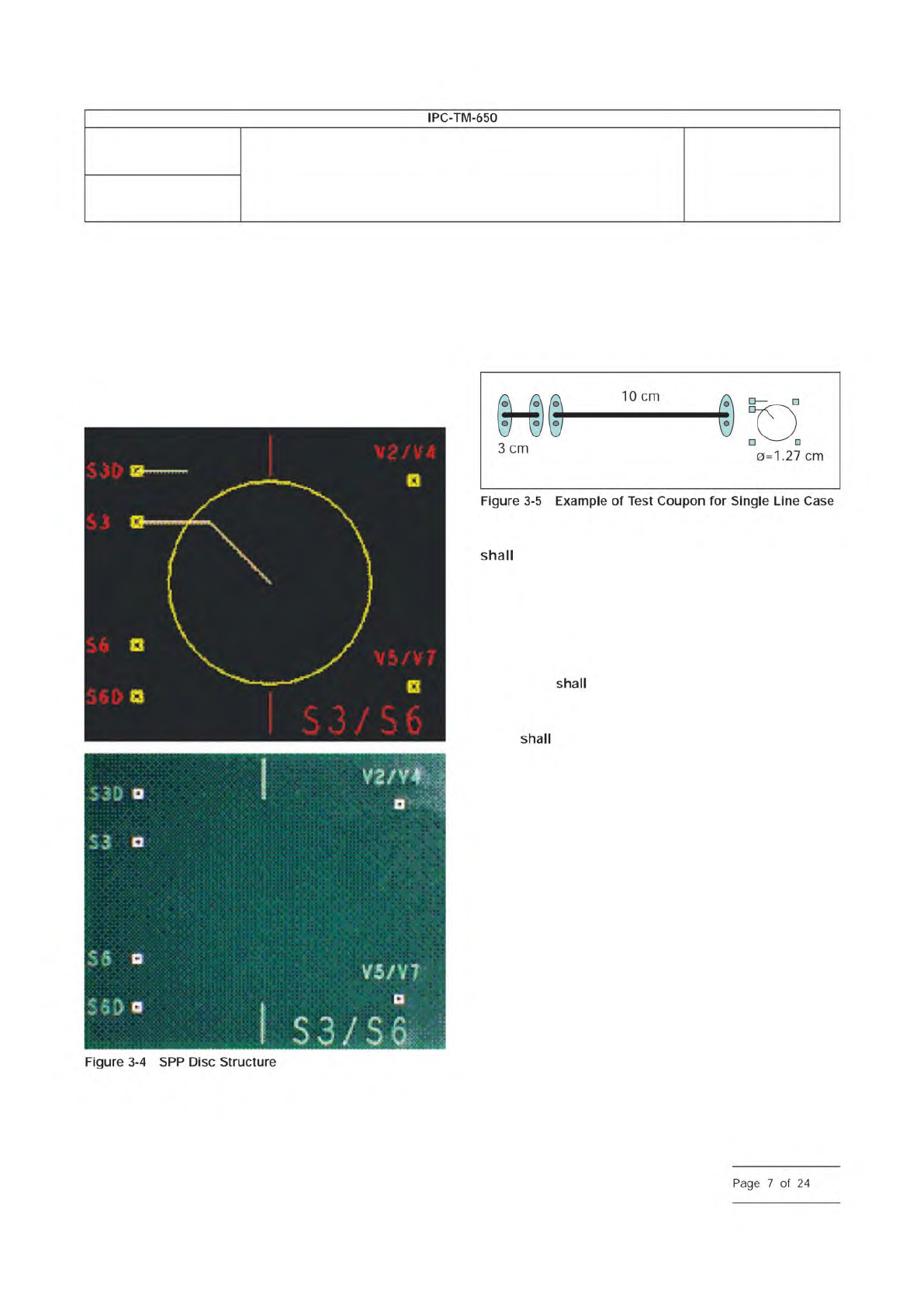
The layout of the disc structure is shown in Figure 3-4. The
red text is on the external surface for pad identification pur-
poses. In a multi-signal layer cross section, disks can be
‘‘stacked’’ vertically to facilitate later cross-sectioning if
desired (e.g., the disc for layer 6 is directly under the disc for
layer 3). The voltage planes around each disc are connected
together at the reference PTH and isolated from the rest of the
test vehicle through the use of a voltage divider.
3.3.4.3 SPP Test Coupon Design
An example is shown of
a typical coupon layout with 3 cm and 10 cm [1.18 in and
3.94 in] long lines and the 12.7 mm [0.5 in] disc in Figure 3-5.
The contacts are shown using the SMA connectors described
in Figure 3-3. This is a minimum configuration. Additional lines
would need to be added for differential line testing. The layout
in Figure 3-5 requires 2.0 cm x 16 cm [0.8 in x 6.3 in] of card
space.
3.3.5 SET2DIL Test Lines
The SET2DIL test coupons
contain one DUT (Device Under Test) for each
impedance/layer combination being controlled, and a ‘‘thru’’
reference structure.
3.3.6 FD Test Lines
The FD test sample shall contain one
transmission (or interconnect) test line per layer. The reference
line shall be between 1.27 cm [0.5 in] and 2.54 cm [1 in].
The test line
be between 15.24 cm [6 in] and 30.49 cm
[12 in]. The recommended line is 1.27 cm [0.5 in] for the ref-
erence line and 20.32 cm [8 in] for the test line. The specific
length be specified by printed board customers or ven-
dors.
3.3.7 Surface Finish
No matter what surface finish is
used, one should ensure the surface of the launch/capture
structure is clean and that the contact of the probes is not
affected by residues and/or oxides. OSP (organic solderability
preservative) finishes may inhibit probing of fine-pitched
probes and may need to be removed from the probe area.
In the lab based qualification/verification assessment, one can
facilitate this by slight burnishing (a pencil eraser often works
well), followed by cleaning with isopropyl alcohol (IPA).
In production floor assessments, the probe design should be
designed to break through any potential oxides or contami-
nants.
4 Apparatus
4.1 Differential and Single Ended Measurements
Both
single ended and differential measurement can be applied to
all the test methods. The measurement process for a differen-
tial measurement is identical to that of a single ended test. For
IPC-25512-3-5
Number
2.5.5.12
Subject
Test Methods to Determine the Amount of Signal Loss on
Printed Boards
Date
07/12
Revision
A
IPC-TM-650
Figure
3-4
SPP
Disc
Structure
shall
shall
shall
Page
7
of
24
the RIE, SPP, and EBW methods the differential voltage mea-
surement is used where the single ended measurement is
specified. For SET2DIL, a slightly different algorithm is used
for single-ended (S21) vs. differential (SDD21) signals. For the
FD (VNA) method, SDD21 is used in place of S21.
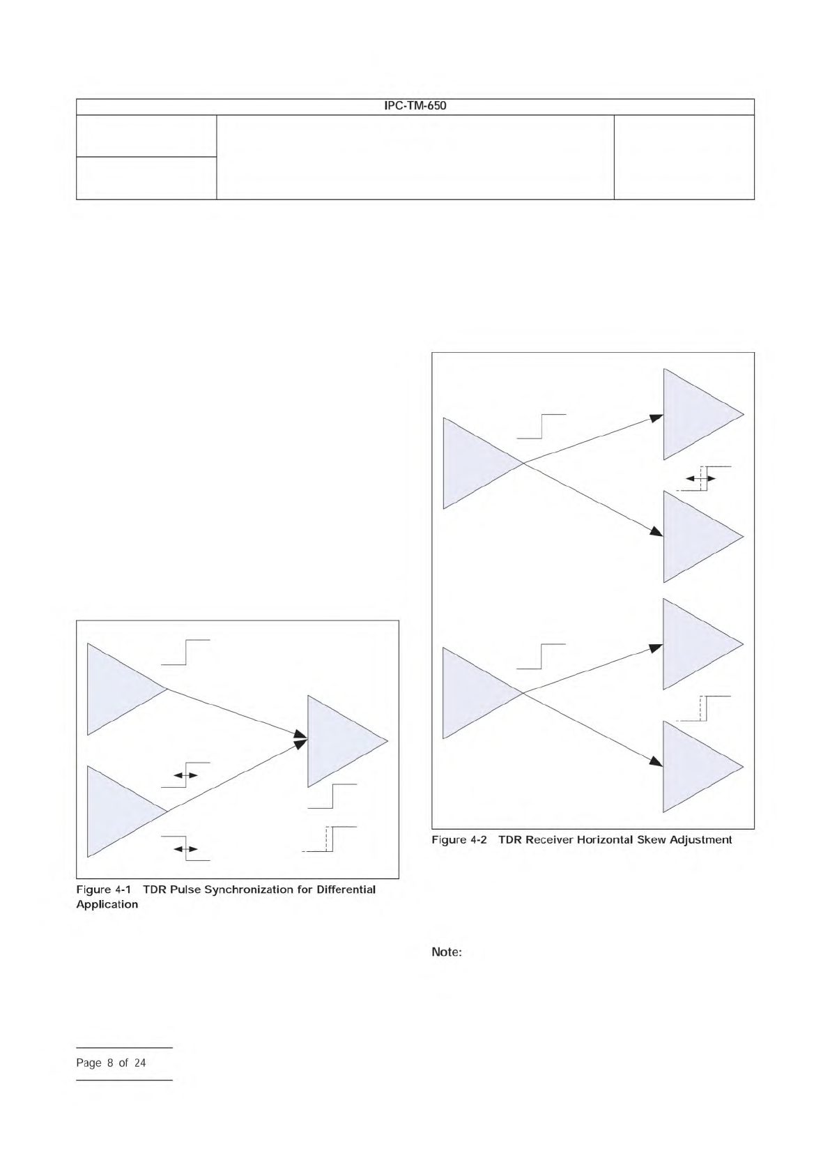
4.1.1 TDR Differential Channel Synchronization
The
two excitation channels need to be synchronized and have
the same amplitude. One recommended method is to use an
oscilloscope that has timing adjustments both in the TDR
heads and in the detector heads. Such a setup is performed
on a short pair of lines or zero-delay configuration. The steps
are as follows:
1) Channel 1 on the source side is propagated and detected
by Channel 3 on the detect side. The pulse or step is
recorded and displayed on the screen. Next, Channel 2 on
the source side is propagated to Channel 3 on the detect
side. The new pulse or step is overlapped with the one on
the screen. If there is a difference, the differential TDR skew
is adjusted until they are coincident. This makes sure that
the two sources do not have any difference in time, as
illustrated in Figure 4-1.
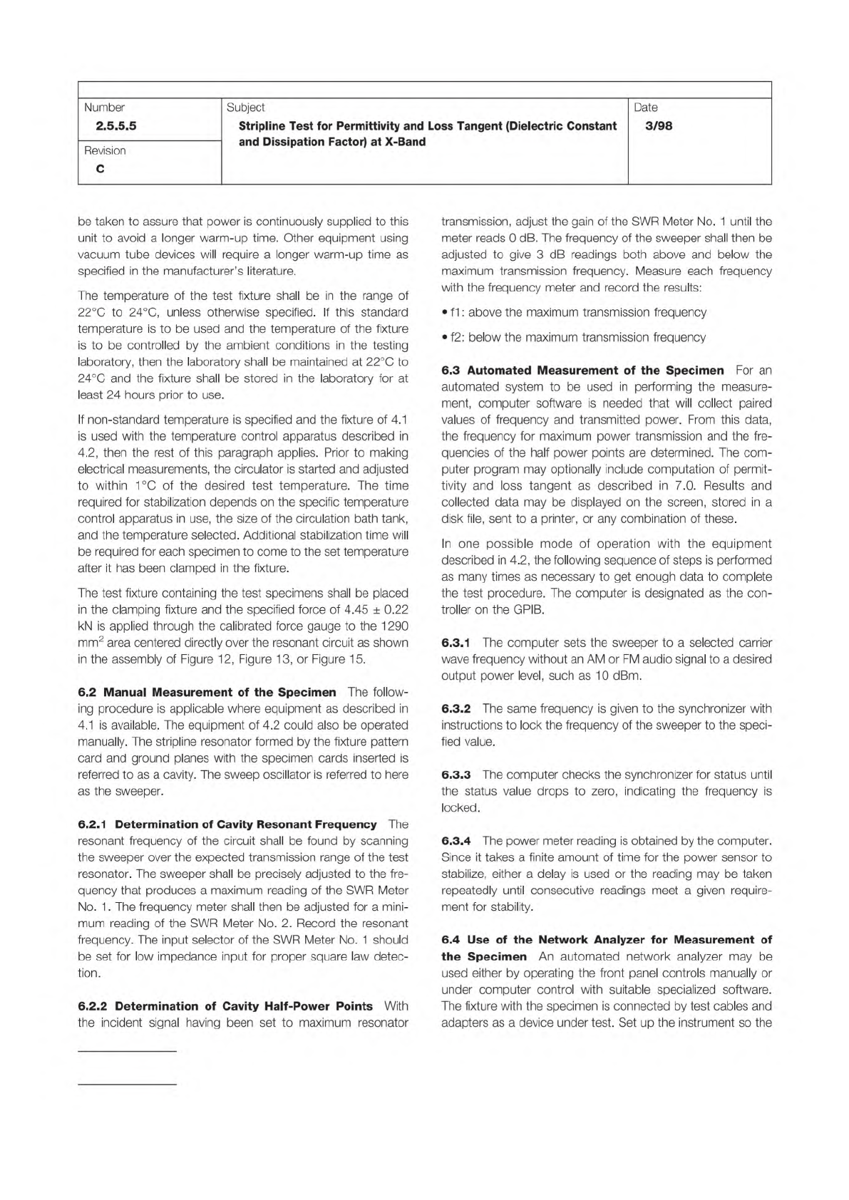
2) Next, the detector channels are adjusted. Channel 1 on the
source side is propagated and detected at this time by
Channel 4 on the detect side. This is compared to the
pulse or step obtained by the path of 1 going into 3. If they
are not synchronized, the Horizontal Skew Adjustment is
used to bring the timings together. Similarly, Channel 3 (or
4) is used as a source into channels 1 & 2; channel 2’s
horizontal skew is adjusted to bring the timings together,
see Figure 4-2. If there is any amplitude difference due to
detector amplification difference, the Channel 4 (or 2)
attenuation can be adjusted to match the waveform of
Channel 3 (or 1).
Both setup steps are needed for TDT and SPP; the first step
alone is enough for TDR used in RIE and EBW; and only step
2 is required for SET2DIL. Step 1 is repeated for Odd-Mode
and for Even-Mode measurements in the differential case.
Channel 2’s excitation must be in the same mode that
will be used during measurements (even or odd) during syn-
chronization; the pulse timing may vary, depending on the
excitation mode. Using a math function to invert the waveform
at the receiver might be necessary for odd mode excitation.
IPC-25512-4-1
1
2
3
IPC-25512-4-2
1
3
4
3
1
2
Number
2.5.5.12
Subject
Test Methods to Determine the Amount of Signal Loss on
Printed Boards
Date
07/12
Revision
A
IPC-TM-650
Note:
Page
8
of
24
IPC-TM-650
Page 6 of 25
Number
2.5.5.5
Subject
Stripline
Test
for
Permittivity
and
Loss
Tangent
(Dielectric
Constant
and
Dissipation
Factor)
at
X-Band
Date
3/98
Revision
C
be
taken
to
assure
that
power
is
continuously
supplied
to
this
unit
to
avoid
a
longer
warm-up
time.
Other
equipment
using
vacuum
tube
devices
will
require
a
longer
warm-up
time
as
specified
in
the
manufacturer's
literature.
The
temperature
of
the
test
fixture
shall
be
in
the
range
of
22℃
to
24℃,
unless
otherwise
specified.
If
this
standard
temperature
is
to
be
used
and
the
temperature
of
the
fixture
is
to
be
controlled
by
the
ambient
conditions
in
the
testing
laboratory,
then
the
laboratory
shall
be
maintained
at
22℃
to
24℃
and
the
fixture
shall
be
stored
in
the
laboratory
for
at
least
24
hours
prior
to
use.
If
non-standard
temperature
is
specified
and
the
fixture
of
4.1
is
used
with
the
temperature
control
apparatus
described
in
4.2,
then
the
rest
of
this
paragraph
applies.
Prior
to
making
electrical
measurements,
the
circulator
is
started
and
adjusted
to
within
1
℃
of
the
desired
test
temperature.
The
time
required
for
stabilization
depends
on
the
specific
temperature
control
apparatus
in
use,
the
size
of
the
circulation
bath
tank,
and
the
temperature
selected.
Additional
stabilization
time
will
be
required
for
each
specimen
to
come
to
the
set
temperature
after
it
has
been
clamped
in
the
fixture.
The
test
fixture
containing
the
test
specimens
shall
be
placed
in
the
clamping
fixture
and
the
specified
force
of
4.45
土
0.22
kN
is
applied
through
the
calibrated
force
gauge
to
the
1290
mm2
area
centered
directly
over
the
resonant
circuit
as
shown
in
the
assembly
of
Figure
12,
Figure
13,
or
Figure
15.
6.2
Manual
Measurement
of
the
Specimen
The
follow¬
ing
procedure
is
applicable
where
equipment
as
described
in
4.1
is
available.
The
equipment
of
4.2
could
also
be
operated
manually.
The
stripline
resonator
formed
by
the
fixture
pattern
card
and
ground
planes
with
the
specimen
cards
inserted
is
referred
to
as
a
cavity.
The
sweep
oscillator
is
referred
to
here
as
the
sweeper.
6.2.1
Determination
of
Cavity
Resonant
Frequency
The
resonant
frequency
of
the
circuit
shall
be
found
by
scanning
the
sweeper
over
the
expected
transmission
range
of
the
test
resonator.
The
sweeper
shall
be
precisely
adjusted
to
the
fre¬
quency
that
produces
a
maximum
reading
of
the
SWR
Meter
No.
1
.
The
frequency
meter
shall
then
be
adjusted
for
a
mini¬
mum
reading
of
the
SWR
Meter
No.
2.
Record
the
resonant
frequency.
The
input
selector
of
the
SWR
Meter
No.
1
should
be
set
for
low
impedance
input
for
proper
square
law
detec¬
tion.
6.2.2
Determination
of
Cavity
Half-Power
Points
With
the
incident
signal
having
been
set
to
maximum
resonator
transmission,
adjust
the
gain
of
the
SWR
Meter
No.
1
until
the
meter
reads
0
dB.
The
frequency
of
the
sweeper
shall
then
be
adjusted
to
give
3
dB
readings
both
above
and
below
the
maximum
transmission
frequency.
Measure
each
frequency
with
the
frequency
meter
and
record
the
results:
•
f1:
above
the
maximum
transmission
frequency
•
f2:
below
the
maximum
transmission
frequency
6.3
Automated
Measurement
of
the
Specimen
For
an
automated
system
to
be
used
in
performing
the
measure¬
ment,
computer
software
is
needed
that
will
collect
paired
values
of
frequency
and
transmitted
power.
From
this
data,
the
frequency
for
maximum
power
transmission
and
the
fre¬
quencies
of
the
half
power
points
are
determined.
The
com¬
puter
program
may
optionally
include
computation
of
permit¬
tivity
and
loss
tangent
as
described
in
7.0.
Results
and
collected
data
may
be
displayed
on
the
screen,
stored
in
a
disk
file,
sent
to
a
printer,
or
any
combination
of
these.
In
one
possible
mode
of
operation
with
the
equipment
described
in
4.2,
the
following
sequence
of
steps
is
performed
as
many
times
as
necessary
to
get
enough
data
to
complete
the
test
procedure.
The
computer
is
designated
as
the
con¬
troller
on
the
GPIB.
6.3.1
The
computer
sets
the
sweeper
to
a
selected
carrier
wave
frequency
without
an
AM
or
FM
audio
signal
to
a
desired
output
power
level,
such
as
10
dBm.
6.3.2
The
same
frequency
is
given
to
the
synchronizer
with
instructions
to
lock
the
frequency
of
the
sweeper
to
the
speci¬
fied
value.
6.3.3
The
computer
checks
the
synchronizer
for
status
until
the
status
value
drops
to
zero,
indicating
the
frequency
is
locked.
6.3.4
The
power
meter
reading
is
obtained
by
the
computer.
Since
it
takes
a
finite
amount
of
time
for
the
power
sensor
to
stabilize,
either
a
delay
is
used
or
the
reading
may
be
taken
repeatedly
until
consecutive
readings
meet
a
given
require¬
ment
for
stability.
6.4
Use
of
the
Network
Analyzer
for
Measurement
of
the
Specimen
An
automated
network
analyzer
may
be
used
either
by
operating
the
front
panel
controls
manually
or
under
computer
control
with
suitable
specialized
software.
The
fixture
with
the
specimen
is
connected
by
test
cables
and
adapters
as
a
device
under
test.
Set
up
the
instrument
so
the