IPC-TM-650 EN 2022 试验方法--.pdf - 第459页
Figure 1 Exploded End Views of Stacked Specimen T y pes A, B, C and D (S ee 3.0) with Copper Foil Thickness Exaggerated and Including the Copper Plates (See 5.1 .2) and Steel Bars (Se e 5.1.1) of the F ixture IPC-TM-650 …

IPC-MF-150
IPC-TM-650
Material in this Test Methods Manual was voluntarily established by Technical Committees of the IPC. This material is advisory only
and its use or adaptation is entirely voluntary. IPC disclaims all liability of any kind as to the use, application, or adaptation of this
material. Users are also wholly responsible for protecting themselves against all claims or liabilities for patent infringement.
Equipment referenced is for the convenience of the user and does not imply endorsement by the IPC.
Page 1 of 11
Number
r
ASSOCIATION
CONNECTING
/
ELECTRONICS
INDUSTRIES
221
5
Sanders
Road
Northbrook,
IL
60062-6135
IPC-TM-650
TEST
METHODS
MANUAL
1
.0
Scope
1.1
Summary
This
method
is
for
measurement
of
relative
permittivity
(er)
and
dissipation
factor
or
loss
tangent
(tan
S)
of
circuit
board
substrates
under
stripline
conditions.
Measure¬
ments
are
made
by
measuring
resonances
of
a
length
of
strip¬
line
over
a
wide
frequency
range
from
below
1
GHz
to
about
14
GHz(1,2).
The
method
permits
a
wide
variety
of
specimen
configurations,
varying
in
dielectric
thickness,
width
of
center
conductor,
and
use
of
clad
or
laid
up
conductor
foil(3).
Sensi¬
tivity
to
differences
in
tan
8
are
enhanced
by
the
ability
to
adjust
the
degree
of
coupling
to
the
resonator
by
adjusting
an
air
gap
between
probes
and
the
resonator
ends.
Many
of
the
principles
used
in
IPC-TM-650,
Method
255.5,
are
applied
in
this
method.
1.2
Terminology
Terms
used
in
this
method
include:
Complex
Relative
Permittivity
―
The
values
for
relative
permit¬
tivity
and
dissipation
factor
considered
as
a
complex
number.
Permittivity
—
Dielectric
constant
(see
IPC-T-50)
or
relative
per¬
mittivity.
The
symbol
used
in
this
document
is
er.
K'
or
k
are
also
sometimes
used.
Relative
Permittivity
—
A
dimensionless
ratio
of
absolute
per¬
mittivity
of
a
dielectric
to
the
absolute
permittivity
of
a
vacuum.
Loss
Tangent
—
Dissipation
factor
(see
IPC-T-50),
dielectric
loss
tangent
(see
9.2).
The
symbol
used
in
this
document
is
tan
8.
1.3
Limitations
The
limitations
in
described
in
1
.3.1
through
1.3.4
should
be
noted.
1.3.1
The
measured
effective
permittivity
for
the
resonator
element
can
differ
from
that
observed
in
an
application.
Where
the
application
is
in
stripline
and
the
line
width
to
ground
plane
spacing
is
less
than
that
of
the
resonator
ele¬
ment
in
the
test,
the
application
will
exhibit
a
greater
compo¬
nent
of
the
electric
field
in
the
X,
Y
plane.
Heterogeneous
dielectric
composites
are
anisotropic
to
some
degree,
result¬
ing
in
a
higher
observed
er
for
narrower
lines.
Microstrip
lines
in
an
application
may
also
differ
from
the
test
in
the
fraction
of
substrate
electric
field
component
in
the
X,
Y
plane.
2.5.5.5.1
Subject
Stripline
Test
for
Complex
Relative
Permittivity
of
Circuit
Board
Materials
to
14
GHz
Date
Revision
3/98
Originating
Task
Group
High
Speed/High
Frequency
Test
Methods
Subcommittee
(D-24)
Bonded
stripline
assemblies
have
air
excluded
between
boards
and
thus
tend
to
show
greater
8r
values
than
would
be
obtained
with
this
method
using
specimen
types
A
or,
to
lesser
extent,
B,
as
discussed
in
3.0.
1.3.2
As
with
IPC-TM-650,
Method
2.
5.
5.5,
with
specimen
type
A,
or,
to
a
lesser
extent,
with
B
(see
3.0),
we
expect
the
method
to
show
a
downward
bias
in
measured
er.
This
is
caused
by
the
electric
field
crossing
clamped
dielectric¬
conductor
interfaces
with
air
included
in
the
surface
rough¬
ness.
1.3.3
With
specimen
type
B,
C,
or
D,
the
method
shows
an
upward
bias
in
measured
tan
5.
This
is
caused
by
the
surface
roughness
and/or
surface
treatment
of
the
clad
copper
foil
required
for
adequate
adhesion
to
the
dielectric.
1.3.4
Compared
to
IPC-TM-650,
Method
2.
5.5.
5,
both
done
with
computer
automated
data
collection,
this
method
requires
a
greater
degree
of
operator
skill
and
more
time
to
prepare
specimens
and
perform
measurements.
1.4
Advantages
1.4.1
The
sensitivity
of
the
method
to
differences
in
er
of
specimens
should
be
superior
to
that
of
IPC-TM-650,
Method
255.5
since
the
specimen
comprises
all
of
the
dielectric
affecting
the
measurement.
1
.4.2
The
method
is
known
to
be
more
sensitive
to
differ¬
ences
in
tan
8
than
IPC-TM-650,
Method
2.5.55
We
believe
the
ability
to
adjust
the
degree
of
probe-to-resonator
coupling
to
a
low
enough
value
that
Q,oaded
is
close
to
Qun|Oaded
(see
7.2.2)
makes
this
possible.
1
.4.3
The
method
is
expected
to
lend
itself
to
use
of
stable
referee
specimens
of
known
electric
properties
traceable
to
NIST
(National
Institute
of
Standards
and
Technology).
2
.0
Applicable
Documents
Metal
Foil
for
Printed
Wiring
Applications
Method
2.
5.5.
5,
Stripline
Test
for
Permittivity
and
Loss
Tangent
(Dielectric
Constant
and
Dissipation
Factor)
at
X-Band
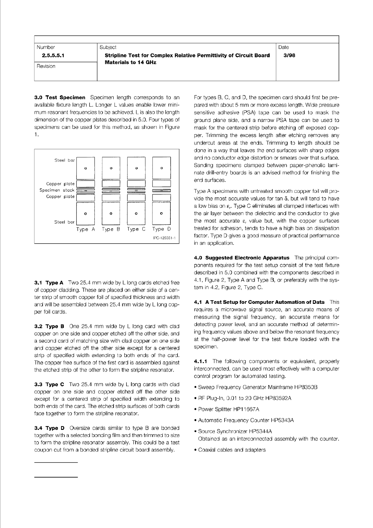
Figure 1 Exploded End Views of Stacked Specimen
Types A, B, C and D (See 3.0) with Copper Foil Thickness
Exaggerated and Including the Copper Plates (See 5.1.2)
and Steel Bars (See 5.1.1) of the Fixture
IPC-TM-650
Page 2 of 11
Number
2.5.5.5.1
Subject
Stripline
Test
for
Complex
Relative
Permittivity
of
Circuit
Board
Materials
to
14
GHz
Date
3/98
Revision
3.0
Test
Specimen
Specimen
length
corresponds
to
an
available
fixture
length
L.
Longer
L
values
enable
lower
mini¬
mum
resonant
frequencies
to
be
achieved.
L
is
also
the
length
dimension
of
the
copper
plates
described
in
5.0.
Four
types
of
specimens
can
be
used
for
this
method,
as
shown
in
Figure
1.
Steel
bar
Copper
plate
0
o
o
o
Specimen
stack
—
-
—
=
.=
Copper
plate
Steel
bar
0
Type
A
0
Type
E
0
Type
C
0
Type
D
I
PC-1
2555
1-1
For
types
B,
C,
and
D,
the
specimen
card
should
first
be
pre¬
pared
with
about
5
mm
or
more
excess
length.
Wide
pressure
sensitive
adhesive
(PSA)
tape
can
be
used
to
mask
the
ground
plane
side,
and
a
narrow
PSA
tape
can
be
used
to
mask
for
the
centered
strip
before
etching
off
exposed
cop¬
per.
Trimming
the
excess
length
after
etching
removes
any
undercut
areas
at
the
ends.
Trimming
to
length
should
be
done
in
a
way
that
leaves
the
end
surfaces
with
sharp
edges
and
no
conductor
edge
distortion
or
smears
over
that
surface.
Sanding
specimens
clamped
between
paper-phenolic
lami¬
nate
drill-entry
boards
is
an
advised
method
for
finishing
the
end
surfaces.
Type
A
specimens
with
untreated
smooth
copper
foil
will
pro¬
vide
the
most
accurate
values
for
tan
6,
but
will
tend
to
have
a
low
bias
on
£r.
Type
0
eliminates
all
clamped
interfaces
with
the
air
layer
between
the
dielectric
and
the
conductor
to
give
the
most
accurate
er
value
but,
with
the
copper
surfaces
treated
for
adhesion,
tends
to
have
a
high
bias
on
dissipation
factor.
Type
D
gives
a
good
measure
of
practical
performance
in
an
application.
3.1
Type
A
Two
25.4
mm
wide
by
L
long
cards
etched
free
of
copper
cladding.
These
are
placed
on
either
side
of
a
cen¬
ter
strip
of
smooth
copper
foil
of
specified
thickness
and
width
and
will
be
assembled
between
25.4
mm
wide
by
L
long
cop¬
per
foil
cards.
3.2
Type
B
One
25.4
mm
wide
by
L
long
card
with
clad
copper
on
one
side
and
copper
etched
off
the
other
side,
and
a
second
card
of
matching
size
with
clad
copper
on
one
side
and
copper
etched
off
the
other
side
except
for
a
centered
strip
of
specified
width
extending
to
both
ends
of
the
card.
The
copper
free
surface
of
the
first
card
is
assembled
against
the
etched
strip
of
the
other
to
form
the
stripline
resonator.
3.3
Type
C
Two
25.4
mm
wide
by
L
long
cards
with
clad
copper
on
one
side
and
copper
etched
off
the
other
side
except
for
a
centered
strip
of
specified
width
extending
to
both
ends
of
the
card.
The
etched
strip
surfaces
of
both
cards
face
together
to
form
the
stripline
resonator.
3.4
Type
D
Oversize
cards
similar
to
type
B
are
bonded
together
with
a
selected
bonding
film
and
then
trimmed
to
size
to
form
the
stripline
resonator
assembly.
This
could
be
a
test
coupon
cut
from
a
bonded
stripline
circuit
board
assembly.
4.0
Suggested
Electronic
Apparatus
The
principal
com¬
ponents
required
for
the
test
setup
consist
of
the
test
fixture
described
in
5.0
combined
with
the
components
described
in
4.1
,
Figure
2,
Type
A
and
Type
B,
or
preferably
with
the
sys¬
tem
in
4.2,
Figure
2,
Type
C.
4.1
A
Test
Setup
for
Computer
Automation
of
Data
This
requires
a
microwave
signal
source,
an
accurate
means
of
measuring
the
signal
frequency,
an
accurate
means
for
detecting
power
level,
and
an
accurate
method
of
determin¬
ing
frequency
values
above
and
below
the
resonant
frequency
at
the
half-power
level
for
the
test
fixture
loaded
with
the
specimen.
4.1.1
The
following
components
or
equivalent,
properly
interconnected,
can
be
used
most
effectively
with
a
computer
control
program
for
automated
testing.
•
Sweep
Frequency
Generator
Mainframe
HP8350B
•
RF
Plug-In,
0.01
to
20
GHz
HP83592A
•
Power
Splitter
HP1
1
667A
•
Automatic
Frequency
Counter
HP5343A
•
Source
Synchronizer
HP5344A
Obtained
as
an
interconnected
assembly
with
the
counter.
•
Coaxial
cables
and
adapters
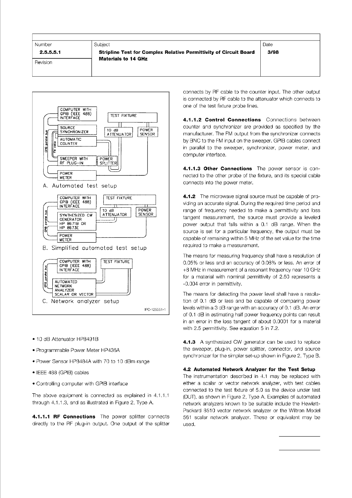
Figure 2 Schematic Drawings of Instrumentation
Setups Suitable for Measurements of Permittivity
IPC-TM-650
Page 3 of 11
Number
2.5.5.5.1
Subject
Stripline
Test
for
Complex
Relative
Permittivity
of
Circuit
Board
Materials
to
14
GHz
Date
3/98
Revision
COMPUTER
WITH
GPIB
(IEEE
438)
INTERFACE
SOURCE
SYNCHRONIZER
AUTOMATIC
COUNTER
SWEEPER
WITH
RF
PLUG-IN
POWER
METER
POWER
SPUTTER
A.
Automated
test
setup
B.
Simplified
automated
test
setup
C.
Network
analyzer
setup
I
PC-1
25551-1
•
10
dB
Attenuator
HP8491
B
•
Programmable
Power
Meter
HP436A
•
Power
Sensor
HP8484A
with
70
to
10
dBm
range
•
IEEE
488
(GPIB)
cables
•
Controlling
computer
with
GPIB
interface
The
above
equipment
is
connected
as
explained
in
4.1
.1
.1
through
4.1
.1
.3,
and
as
illustrated
in
Figure
2,
Type
A.
4.
1.1.1
RF
Connections
The
power
splitter
connects
directly
to
the
RF
plug-in
output.
One
output
of
the
splitter
connects
by
RF
cable
to
the
counter
input.
The
other
output
is
connected
by
RF
cable
to
the
attenuator
which
connects
to
one
of
the
test
fixture
probe
lines.
4.1
.1
.2
Control
Connections
Connections
between
counter
and
synchronizer
are
provided
as
specified
by
the
manufacturer.
The
FM
output
from
the
synchronizer
connects
by
BNC
to
the
FM
input
on
the
sweeper.
GPIB
cables
connect
in
parallel
to
the
sweeper,
synchronizer,
power
meter,
and
computer
interface.
4.
1.1.3
Other
Connections
The
power
sensor
is
con¬
nected
to
the
other
probe
of
the
fixture,
and
its
special
cable
connects
into
the
power
meter.
4.1.2
The
microwave
signal
source
must
be
capable
of
pro¬
viding
an
accurate
signal.
During
the
required
time
period
and
range
of
frequency
needed
to
make
a
permittivity
and
loss
tangent
measurement,
the
source
must
provide
a
leveled
power
output
that
falls
within
a
0.1
dB
range.
When
the
source
is
set
for
a
particular
frequency,
the
output
must
be
capable
of
remaining
within
5
MHz
of
the
set
value
for
the
time
required
to
make
a
measurement.
The
means
for
measuring
frequency
shall
have
a
resolution
of
0.05%
or
less
and
an
accuracy
of
0.08%
or
less.
An
error
of
+8
MHz
in
measurement
of
a
resonant
frequency
near
1
0
GHz
for
a
material
with
nominal
permittivity
of
2.50
represents
a
-0.004
error
in
permittivity.
The
means
for
detecting
the
power
level
shall
have
a
resolu¬
tion
of
0.1
dB
or
less
and
be
capable
of
comparing
power
levels
within
a
3
dB
range
with
an
accuracy
of
0.1
dB.
An
error
of
0.1
dB
in
estimating
half
power
frequency
points
can
result
in
an
error
in
the
loss
tangent
of
about
0.0001
for
a
material
with
2.5
permittivity.
See
equation
5
in
7.2.
4.1.3
A
synthesized
CW
generator
can
be
used
to
replace
the
sweeper,
plug-in,
power
splitter,
connector,
and
source
synchronizer
for
the
simpler
set-up
shown
in
Figure
2,
Type
B.
4.2
Automated
Network
Analyzer
for
the
Test
Setup
The
instrumentation
described
in
4.1
may
be
replaced
with
either
a
scalar
or
vector
network
analyzer,
with
test
cables
connected
to
the
test
fixture
of
5.0
as
the
device
under
test
(DUT),
as
shown
in
Figure
2,
Type
A.
Examples
of
automated
network
analyzers
known
to
be
suitable
include
the
Hewlett-
Packard
8510
vector
network
analyzer
or
the
Wiltron
Model
561
scalar
network
analyzer.
These
or
equivalent
may
be
used.