IPC-TM-650 EN 2022 试验方法--.pdf - 第502页
h t t p : / / physics.nist.gov/cgi-bin/cuu/V alue?ep0|search_for=permitti vity 6 1 Center conductor pin a = 3.05 mm 2 Supporting dielectric in the APC-7 section 3 Center conductor in the APC-7 to APC-3.5 4 Supporting die…
/
S
/
S
Z
IPC-TM-650
Page 5 of 8
Number
2.5.5.10
Subject
High
Frequency
Testing
to
Determine
Permittivity
and
Loss
Tangent
of
Embedded
Passive
Materials
Date
07/05
Revision
For
each
frequency
repeat
the
following
procedure:
1
.
Compute
the
complex
permittivity
using
Equations
(2b)
and
(2c).
This
is
an
initial
trial
solution
of
the
iterative
process
for
k=0,
where
k
is
the
iterative
step:
£
;
[k
=
0]
=
V
-尤"
(
7b)
2.
Compute
successive
approximations
for
subsequent
itera¬
tive
steps
k.
A
[k
+
1
]
=
<p
(J
[k])
(7c)
(k
=
0,
1
,
2,
3...)
3.
The
iteration
procedure
is
terminated
when
the
absolute
value
of
Equation
(7d)
is
sufficiently
small,
for
example
smaller
than
1
0-5.
|E;W-£;[k-1]|
|e;W|<10-5
(7d)
Typically
it
may
require
five
to
about
twenty
iterations
to
reach
the
terminating
criterion.
Commercially
available
software
can
be
used
to
program
and
automate
the
computational
steps
1
through
3
and
solve
Equation
(7)
numerically
for
e*
and
the
corresponding
uncer¬
tainty
values.
The
software
should
be
capable
of
handling
simultaneously
both
real
and
imaginary
parts
of
complex
〕
〔
,
x
cot
(x)
and
£*,
(for
example
Visual
Basic,
C
or
Agilent
VEE
and
National
Instruments
LabView
programming
platforms
can
be
employed).
8
Report
The
report
shall
include:
•
Dimensions
of
the
specimen.
•
Plot
of
magnitude
and
phase
of
the
measured
impedance
as
a
function
of
frequency,
(similar
to
Figure
3)
or
Smith
Chart.
•
Plot
of
£'
and
U'
or
ez
and
tan
8
as
a
function
of
frequency.
9
Notes
9.1
Measurements
at
Frequency
Range
Above
12
GHz
The
presented
APC-7
test
fixture
design
may
be
utilized
in
the
frequency
range
of
100
kHz
to
18
GHz.
The
computational
algorithm
and
in
particular
Equations
(4)
and
(5)
have
been
validated
up
to
the
first
cavity
resonance
frequency,
fcav,
which
is
determined
by
the
propagation
length
/,
and
the
dielectric
constant
of
the
specimen:
fcav
=
^-7=
~
1
21
N%
[GHz]
I
Re
(\e^)
(8)
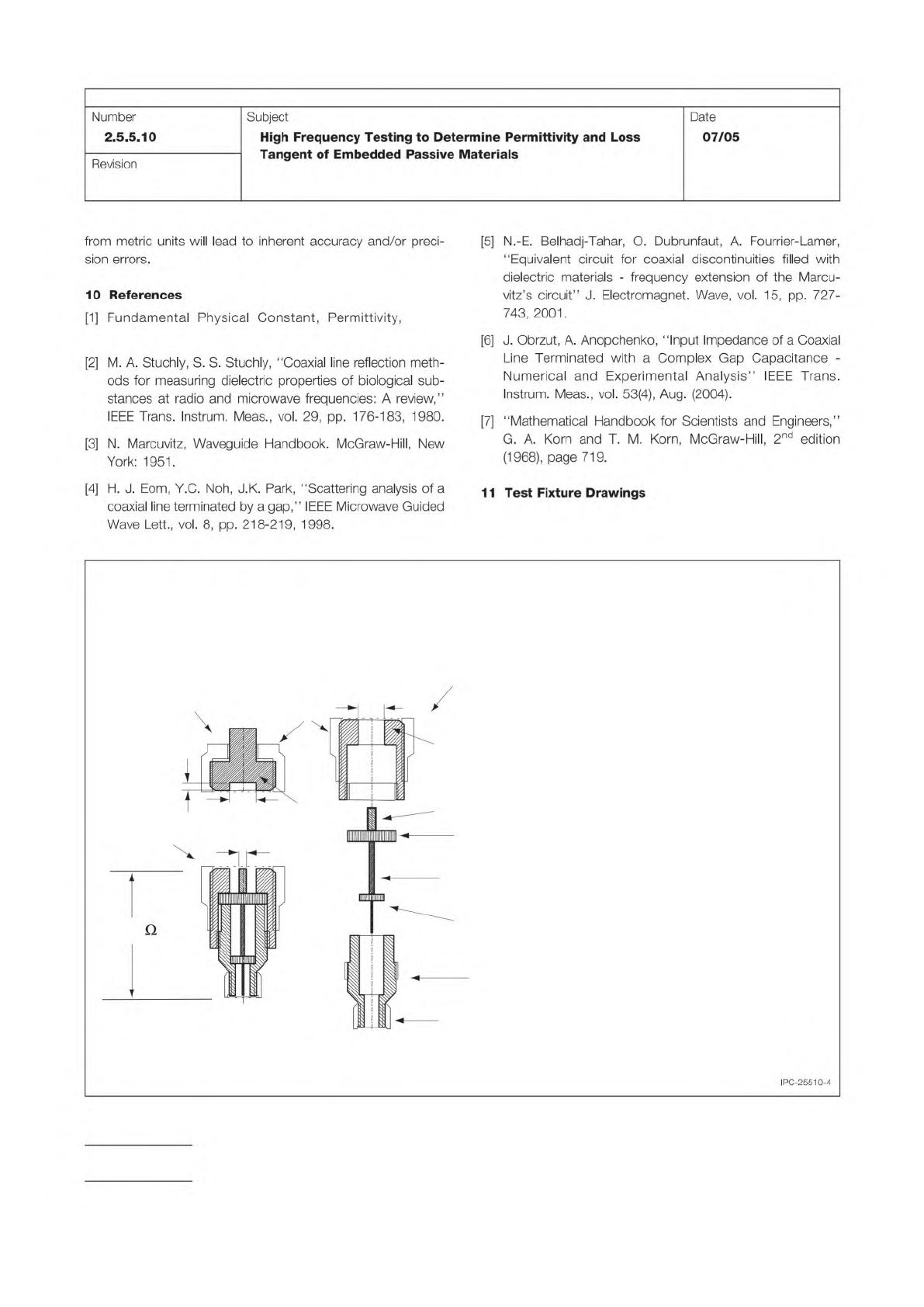
where
Re
indicates
the
real
part
of
complex
square
root
of
permittivity
and
/
=
2.47
mm,
which
is
the
propagation
length
for
the
test
fixture
presented
in
Figure
1,
[5].
For
example,
in
the
case
of
a
specimen
having
the
dielectric
constant
of
1
00
fcav
is
about
1
2
GHz.
9.2
Accuracy
Considerations
Several
uncertainty
factors
such
as
instrumentation,
dimensional
uncertainty
of
the
test
specimen
geometry,
roughness
and
conductivity
of
the
con¬
duction
surfaces
contribute
to
the
combined
uncertainty
of
the
measurements.
The
complexity
of
modeling
these
factors
is
considerably
higher
within
the
frequency
range
of
the
LC
reso¬
nance.
Adequate
analysis
can
be
performed,
however,
by
using
the
partial
derivative
technique
[1]
for
Equations
(2b)
and
(2c)
and
considering
the
instrumentation
and
the
dimensional
errors.
The
standard
uncertainty
of
「
can
be
assumed
to
be
within
the
manufacturer's
specification
for
the
network
ana¬
lyzer,
about
±
0.005
dB
for
the
magnitude
and
土
0.5°
for
the
phase.
The
combined
relative
standard
uncertainty
in
geo¬
metrical
capacitance
measurements
is
typically
better
than
5%,
where
the
largest
contributing
factor
is
the
uncertainty
in
the
film
thickness
measurements.
Equation
(5)
for
the
residual
inductance
has
been
validated
for
specimens
8
pm
to
300
pm
thick.
However,
since
residual
inductance
becomes
smaller
with
thinner
dielectrics,
mea¬
surements
can
be
accurately
made
for
sample
thicknesses
down
to
1
pm.
Measurements
in
the
frequency
range
of
100
MHz
to
12
GHz
are
reproducible
with
relative
combined
uncertainty
in
£'
and
of
better
than
8%
for
specimens
having
e(
<80
and
thick¬
ness
d
<300
pm.
The
resolution
in
the
dielectric
loss
tangent
measurements
is
<0.005.
Additional
limitations
may
arise
from
the
systematic
uncer¬
tainty
of
the
particular
instrumentation,
calibration
standards
and
the
dimensional
imperfections
of
the
actually
imple¬
mented
test
fixture.
Results
may
be
not
reliable
at
frequencies
where
| |
decreases
below
0.05
Q,
which
in
Figure
3
is
shown
as
a
frequency
range
of
11
.9
GHz
to
1
3.5
GHz.
9.3
Test
Software
Test
software
enabling
this
technique
to
be
performed
is
available
in
the
Agilent
VEE
platform.
Please
contact
Dr.
Jan
Obrzut
at
NIST-Gaithersburg,
MD
(jan.obrzut@nist.gov)
to
obtain
such.
9.4
Metric
Units
of
Measure
This
test
method
uses
only
metric
units
of
measure,
as
is
the
case
with
nearly
all
such
high
frequency
test
methods.
Conversion
to
English/lmperial
units
has
not
been
done
in
this
document,
as
any
conversions
http://
physics.nist.gov/cgi-bin/cuu/Value?ep0|search_for=permittivity
6
1 Center conductor pin
a
= 3.05 mm
2 Supporting dielectric in the APC-7 section
3 Center conductor in the APC-7 to APC-3.5
4 Supporting dielectric in the APC-3.5 section
5 APC-3.5 section of the adaptor
6 Section A outer conductor (
b
=7.00 mm)
7 Section B outer conductor (
b
=7.00 mm)
8 APC-7 mount
8
1
2
a
d
b
b
Section B
Section A
Section A details
Test Fixture for HF Permittivity of Embedded Passive Materials
Originator: IPC Embedded Passives Test Methods
3
4
5
50
Calibration Plane
METRIC, dimensions are in mm
7
APC-3.5 female mount
IPC-TM-650
Page 6 of 8
Number
2.5.5.10
Subject
High
Frequency
Testing
to
Determine
Permittivity
and
Loss
Tangent
of
Embedded
Passive
Materials
Date
07/05
Revision
from
metric
units
will
lead
to
inherent
accuracy
and/or
preci¬
sion
errors.
10
References
[1]
Fundamental
Physical
Constant,
Permittivity,
[2]
M.
A.
Stuchly,
S.
S.
Stuchly,
"Coaxial
line
reflection
meth¬
ods
for
measuring
dielectric
properties
of
biological
sub¬
stances
at
radio
and
microwave
frequencies:
A
review,”
IEEE
Trans.
Instrum.
Meas.,
vol.
29,
pp.
176-183,
1980.
[3]
N.
Marcuvitz,
Waveguide
Handbook.
McGraw-Hill,
New
York:
1951.
[4]
H.
J.
Eom,
Y.C.
Noh,
J.K.
Park,
"Scattering
analysis
of
a
coaxial
line
terminated
by
a
gap,”
IEEE
Microwave
Guided
Wave
Lett.,
vol.
8,
pp.
218-219,
1998.
[5]
N.-E.
Belhadj-Tahar,
O.
Dubrunfaut,
A.
Fourrier-Lamer,
"Equivalent
circuit
for
coaxial
discontinuities
filled
with
dielectric
materials
-
frequency
extension
of
the
Marcu-
vitz's
circuit”
J.
Electromagnet.
Wave,
vol.
15,
pp.
727-
743,
2001.
[6]
J.
Obrzut,
A.
Anopchenko,
'Input
Impedance
of
a
Coaxial
Line
Terminated
with
a
Complex
Gap
Capacitance
-
Numerical
and
Experimental
Analysis”
IEEE
Trans.
Instrum.
Meas.,
vol.
53(4),
Aug.
(2004).
[7]
"Mathematical
Handbook
for
Scientists
and
Engineers,”
G.
A.
Korn
and
T.
M.
Korn,
McGraw-Hill,
2nd
edition
(1968),
page
719.
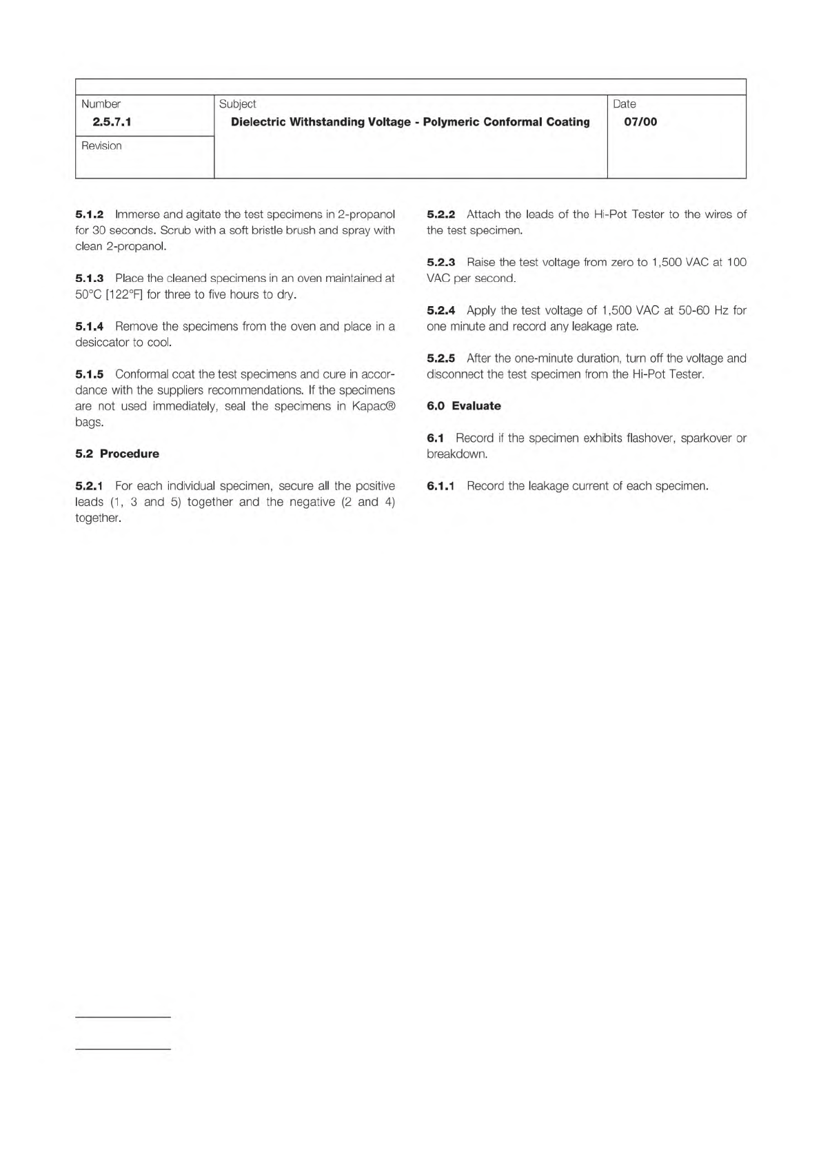
11
Test
Fixture
Drawings
IPC-25510-4
IPC-TM-650
Page 2 of 2
Number
2.5.7.1
Subject
Dielectric
Withstanding
Voltage
-
Polymeric
Conformal
Coating
Date
07/00
Revision
5.1.2
Immerse
and
agitate
the
test
specimens
in
2-propanol
for
30
seconds.
Scrub
with
a
soft
bristle
brush
and
spray
with
clean
2-propanol.
5.1.3
Place
the
cleaned
specimens
in
an
oven
maintained
at
50℃
[1
22°F]
for
three
to
five
hours
to
dry.
5.1.4
Remove
the
specimens
from
the
oven
and
place
in
a
desiccator
to
cool.
5.1.5
Conformal
coat
the
test
specimens
and
cure
in
accor¬
dance
with
the
suppliers
recommendations.
If
the
specimens
are
not
used
immediately,
seal
the
specimens
in
Kapac®
bags.
5.2
Procedure
5.2.1
For
each
individual
specimen,
secure
all
the
positive
leads
(1
,
3
and
5)
together
and
the
negative
(2
and
4)
together.
5.2.2
Attach
the
leads
of
the
Hi-Pot
Tester
to
the
wires
of
the
test
specimen.
5.2.3
Raise
the
test
voltage
from
zero
to
1,500
VAC
at
1
00
VAC
per
second.
5.2.4
Apply
the
test
voltage
of
1
,500
VAC
at
50-60
Hz
for
one
minute
and
record
any
leakage
rate.
5.2.5
After
the
one-minute
duration,
turn
off
the
voltage
and
disconnect
the
test
specimen
from
the
Hi-Pot
Tester.
6.0
Evaluate
6.1
Record
if
the
specimen
exhibits
flashover,
sparkover
or
breakdown.
6.1.1
Record
the
leakage
current
of
each
specimen.