IPC-TM-650 EN 2022 试验方法--.pdf - 第536页
IPC-25512-5-6 0.4 -0.01 0 0.2 0.3 0.1 0 2 4 6 8 10 Measurement Simulation 0.4 -0.01 0 0.2 0.3 0.1 0 2 4 6 8 10 Measurement Simulation Measurement Simulation l = 5 cm l = 8 cm l = 5 cm l = 20 cm T ime (nsec) V oltage (V) …

this case, the screening has to be done for odd-mode, with
TDR pulse polarity of + -, and even-mode, + +. It is also rec-
ommended to perform TDR for +0 and 0+ single mode to see
how close to each other the two lines’ characteristics are.
5.3.2 Measuring Frequency Relative Permittivity with
SPP
The capacitance be measured at 1 MHz with an
LCR meter for several lengths of lines. Such measurements
are generally made at a low enough frequency such as 1 MHz
so that the reactance associated with the lead inductance is
negligible. In a subsequent step line resistance measurements
using a 4 wire Kelvin method are also made. The measure-
ments determine the resistance per unit length and the
capacitance per unit length. By taking the difference between
results at two lengths and dividing by the difference in lengths,
the effect of parasitic end load is eliminated. The LCR meter
be also used to measure the capacitance between the
layers of the large circular disc designated for dielectric per-
mittivity determination.
Relative permittivity, ε
r
, is calculated with Equation 5-6 using
the known area, A, of the test specimen disc, the distance
between the layers h, and the capacitance, C, as measured
with the LCR at 1 MHz. The value for ‘‘h’’ may be determined
by cross-sectioning analysis.
ε
r
=
hC
ε
0
A
[5-6]
5.3.3 Measuring Low Frequency Copper Resistivity, ρ,
with SPP
The resistivity (ρ) per unit length of the signal line
conductor is determined with Equation 5-7. R
l
is the resis-
tance measured using a 4 wire Kelvin method for the long line
of length l
l
. R
s
is the resistance measured using a 4 wire Kel-
vin method for the short line of length l
s
.
ρ =
(R
l
− R
s
)A
l
l
− l
s
[5-7]
A is the cross-section area (equal to the conductor width mul-
tiplied by the conductor thickness).
5.3.4 SPP Low Frequency Permittivity
It should be
noted that the two ground planes that are above and below
the signal of interest are always shorted together, in the trans-
mission line region and in the parallel plate disc area. The disc
that is used should have a diameter that is 100x the height, h
to, the nearest ground in order to be able to calculate ε
r
directly from (1) without any fringe capacitance consideration.
The typical diameter of the disc is 12.7 mm [0.5 in]. It is use-
ful to have a dummy structure that is nearby the disc that has
only the via connection between the surface pad and the disc
and the small lateral line extension. Typical configuration was
shown in 3.3.4.2. The capacitance of this parasitic structure is
subtracted from the total disc C so that the end effects are not
included in the result for ε
r
.
Finally, the dielectric loss, tanδ, is also measured for the large
disc using the same LCR meter in the range of 10 KHz to
1 MHz.
The line capacitance per unit length, together with the cross
sectional dimensions can also be used for determining the
dielectric constant at 1 MHz. The procedure is to calculate the
capacitance with a 2D field solver for an assumed dielectric
constant. Iteration is used on this assumed value until the
agreement is obtained between measured and calculated C.
The implicit assumption here is that the lines are uniform and
that the cross section is well known along the length. Both
these assumptions have limitations and this is why the extrac-
tion based on line C is not as accurate. On the other hand, the
composition of glass fiber and dielectric resin might differ in
the disc area from the line area which could introduce errors
in the extracted ε
r
at 1 MHz.
5.3.5 SPP TDT Measurement
TDT measurements are
also made with several lines, but especially with the 2 cm
[0.787 in] and 8 cm [3.15 in] lines of interest. In addition, it is
useful to measure a very short line of ‘‘zero length,’’ (e.g., 0.25
- 0.45 mm [0.0098 - 0.0177 in]) in order to obtain the band-
width of the time-domain set-up and for use as a reference for
delay extraction. The TDT measurement monitors the propa-
gation delay at 50% of the signal swing, the propagated rise
time between 10% and 90% levels. By taking the difference in
delays for the two lines and dividing by the difference in
lengths, one obtains the line propagation delay per unit length,
τ, without the effect of probes, pads, and via discontinuities.
The assumption is that these features are of similar character-
istics for the two lines. The propagated risetime through the
‘‘zero length’’ line indicates the bandwidth for the setup based
on the simplified formula for the upper 3 dB frequency given
in Equation 5-8.
, =
0.35
tr
[5-8]
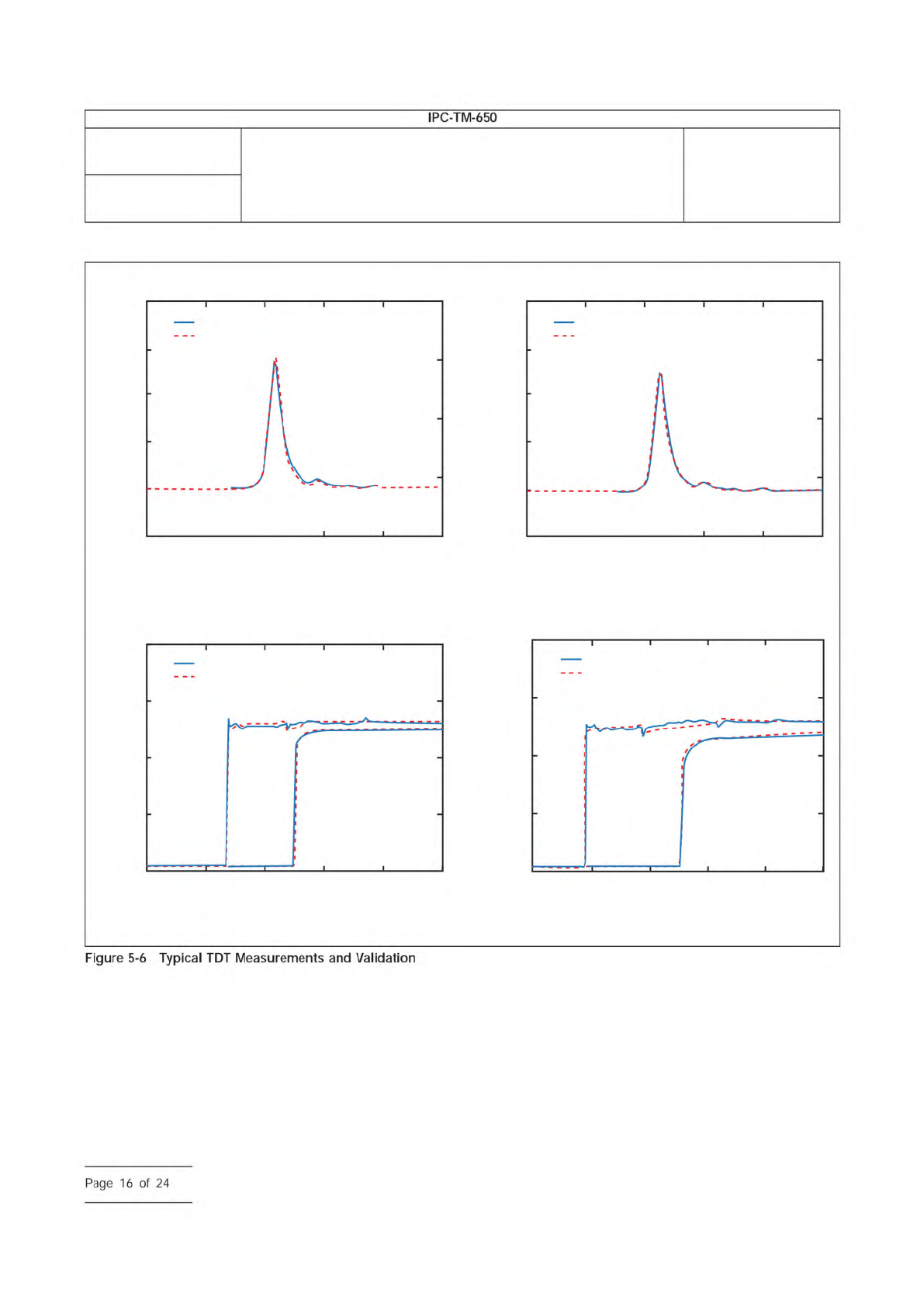
The correlation of propagation delay and rise time shape with
simulation can provide a very useful validation of the broad-
band model that is being created using this method.
Examples are given in Figure 5-6.
Number
2.5.5.12
Subject
Test Methods to Determine the Amount of Signal Loss on
Printed Boards
Date
07/12
Revision
A
IPC-TM-650
shall
shall
Page
15
of
24
IPC-25512-5-6
0.4
-0.01
0
0.2
0.3
0.1
0 2 4 6 8 10
Measurement
Simulation
0.4
-0.01
0
0.2
0.3
0.1
0 2 4 6 8 10
Measurement
Simulation
Measurement
Simulation
l = 5 cm l = 8 cm
l = 5 cm
l = 20 cm
Time (nsec)
Voltage (V)
Time (nsec)
Voltage (V)
Voltage (V)
0.04
-0.01
0.02
0.03
0.01
0 0.2 0.4 0.6 0.8 1
0
Time (nsec)
Measurement
Simulation
Voltage (V)
0.04
-0.01
0.02
0.03
0.01
0 0.2 0.4 0.6 0.8 1
0
Time (nsec)
Number
2.5.5.12
Subject
Test Methods to Determine the Amount of Signal Loss on
Printed Boards
Date
07/12
Revision
A
IPC-TM-650
Figure
5-6
Typical
TDT
Measurements
and
Validation
Page
16
of
24
Both narrow pulse and step-source propagation measure-
ments are compared with the simulations. Dielectric losses
become significant mostly on longer lines, while short duration
pulses propagated on shorter lines highlight the good agree-
ment for the high-frequency fit. The agreement in both cases,
both in timing and signal amplitude and shape, perform the
complete validation. In addition, propagation delay measured
on a medium length line, such as 5 cm where losses are not
very strong and end effects are not too significant, can pro-
vide an approximate calculation of ε
r
. This is an approximate
value because the lines are not ideal, losses are present, and
the signal is broadband. However, it gives a bound on the
value of ε
r
that indicates that the disc extraction is not totally
incorrect. The ideal dielectric is then obtained from Equation
5-9.
τ =
√
ε
r
c
[5-9]
where τ is the propagation delay per unit length obtained from
TDT and c is the speed of light in a vacuum. As indicated
before, printed board technology could have fairly large
dimensional tolerances. This is why it is advisable to perform
as many validations of the extracted material parameters as
possible with various approaches, such as the large disc, the
line C, and the TDT-based delay.
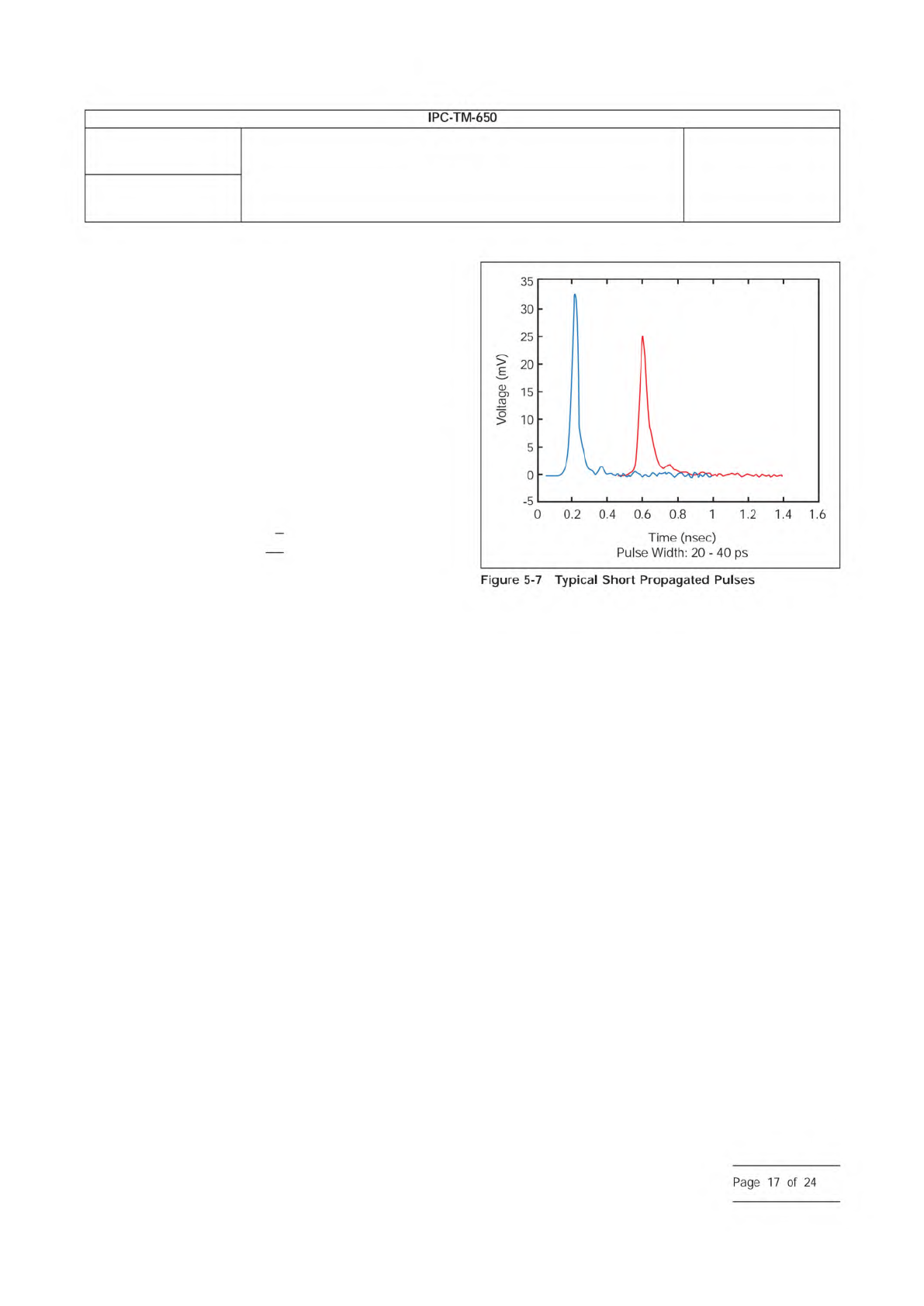
5.3.6 SPP Short-Pulse Measurement
The final type of
electrical measurement is where the technique gets its name.
Pulses of high-frequency content are sent through the con-
ductors, and the output is measured and digitally captured. A
short pulse is created by differentiating a step function. Most
sampling oscilloscopes have suitable step function generation
capability for the general purpose of TDR. Simple passive dif-
ferentiator networks can be placed in-line with the source
cable connecting to the coaxial probes or connectors inject-
ing signal into the printed board. Newer rise time-enhancing
amplifiers can also be placed in-line before the differentiator to
extend the measurement bandwidth. Measurements can be
made with coaxial probes or SMA connector interfaces. A
digitized pulse is measured on each of two lengths of identical
transmission lines. Sample results are shown in Figure 5-7.
Care needs to be taken to use the highest appropriate band-
width cables, probes, adapters; the smallest and shortest
vias, the smallest pads; highest bandwidth detector circuit;
and fastest differentiator (IFN).
Pulses are measured with 512 to 1024 point resolution. The
recommendation is to have 1024 points of timing resolution. It
is acceptable to concatenate captured frames to achieve this.
Typical oscilloscope time base settings are in the range of
25-75 ps/div, depending on the equipment used and length of
lines. The vertical scale is set to maximize use of the screen
while ensuring the entire waveform is captured. It is recom-
mended that captured waveforms consist of 256 averages.
Pulses are generally shifted toward the left of the oscilloscope
screen with just enough of a base DC portion to establish the
correct base reference level. A good rule of thumb is to have
the peak of the pulse reside at the 2nd major horizontal divi-
sion on the screen. The inclusion of the right hand tail of the
signal permits the capture of as much low frequency spectral
content as possible in one frame. The selection of the time per
division setting is then a compromise between having very
high time resolution for the fast portion of the pulse itself and
the need to include the return to ground tail end of the pulse
in less than two frames. The use of more than 1024 horizon-
tal points is not recommended.
The signal line impedance is designed to match the measure-
ment environment of 50 Ω, but this is not absolutely neces-
sary. Different impedances are tolerated, but large differences
may generate too large of an interface reflection that cannot
be eliminated by time-windowing of the Fourier transforms
and could also distort the pulse shapes. The above examples
are considered extremely clean.
The amplitude of the propagated signal should be maximized
through proper contact during probing. If using a probe sta-
tion, this is accomplished through use of proper down force.
IPC-25512-5-7
Number
2.5.5.12
Subject
Test Methods to Determine the Amount of Signal Loss on
Printed Boards
Date
07/12
Revision
A
IPC-TM-650
-5
0
0.2
0.4
0.6
0.8
1
1.2
1.4
1.6
Time
(nsec)
Pulse
Width:
20
-
40
ps
Figure
5-7
Typical
Short
Propagated
Pulses
5
0
5
0
5
0
5
3
3
2
2
1
1
>
E)
o
>
Page
17
of
24