IPC-TM-650 EN 2022 试验方法--.pdf - 第540页
The calc ulation is it erat e d until good ag reement is obtained. Agreement is assessed v isually. Each t ime, the high-freque ncy values of ε r and tan δ ar e modified. It is recommended to use a 2D field so lver that …
V1(f) and V2(t) is a respective ordered frequency pair A1(f),
φ1(f) and A2(f), φ2(f).
The attenuation, Att(f), and phase constant, β(f), are com-
puted with Equations 5-10 and 5-11.
Γ(,) = α(,) + jβ(,) =
−
1
l
1
– l
2
1n
(
A
1
(,)
A
2
(,)
)
+ j
φ
1
(,) − φ
2
(,)
l
1
− l
2
[5-10]
Att(,) = 20 log (e
Re(Γ(,)
)
β(,) = Im (Γ(F))
[5-11]
5.3.6.3 SPP Broadband Complex Permittivity Extraction
5.3.6.3.1 Frequency Dependent Line Parameters
A 2D
field solver is used to calculate R(f), L(f), C(f), and G(f) per unit
length based on the actual cross sectional dimensions, the
metal resistivity ρ, and low frequency ε
r
and tanδ outlined
above. A 2D solver that assures a causally related calculation
of L-R and C-G is recommended. The initial calculation can
contain a few initial points for ε
r
and tanδ that are used as
starting values for the high-frequency range, for example
3 GHz to 20 GHz. Based on the calculated R(f), L(f), C(f), and
G(f), the attenuation and phase constant are calculated from
Equation 5-12.
Γ(,) = α(,) + jβ(,) =
√
(R + jωL)(G + jωC)
[5-12]
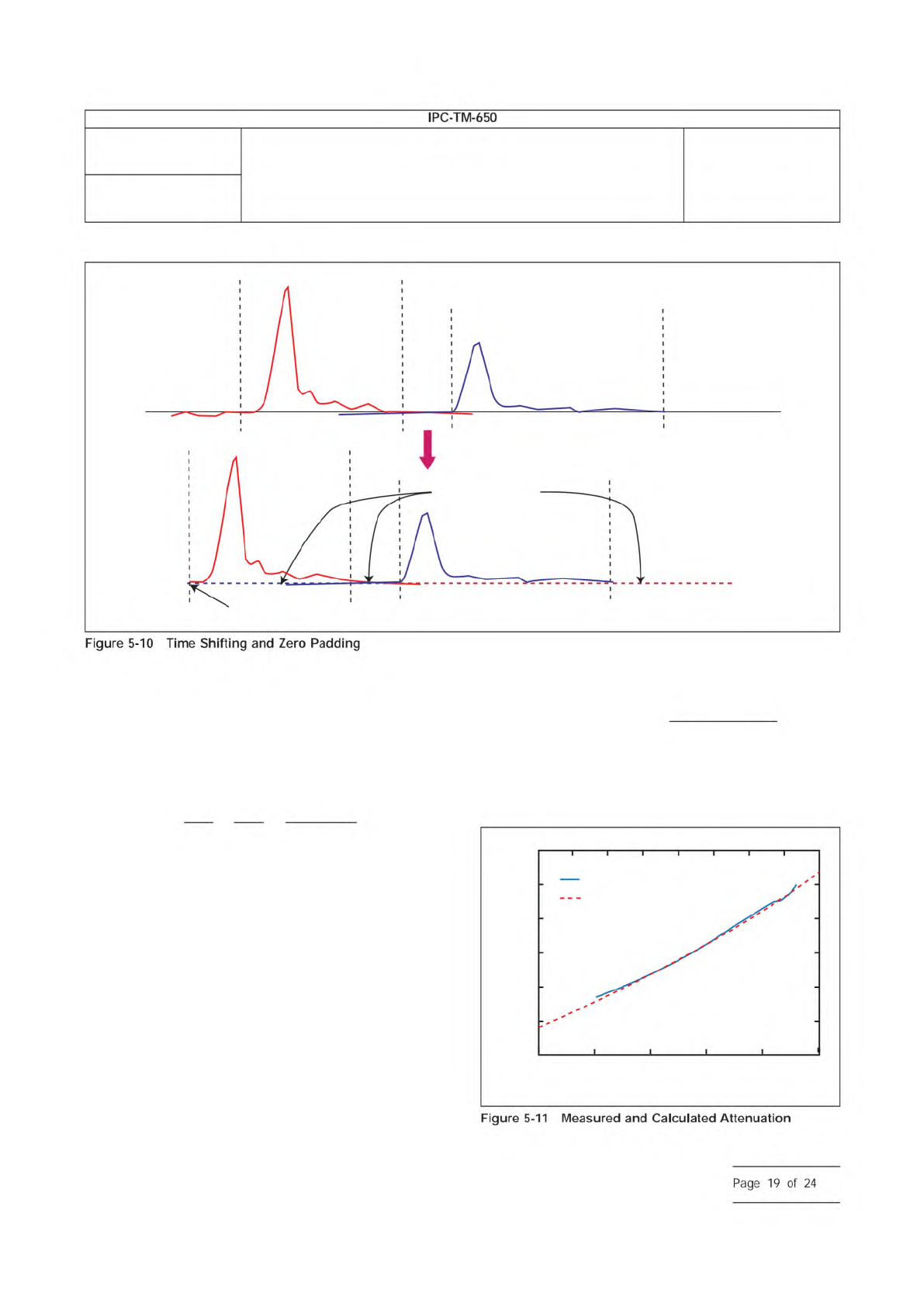
The measured and calculated attenuation and phase are
compared to the measured values as shown in Figure 5-11
and Figure 5-12.
IPC-25512-5-10
0V, 0S
Zero Padded
IPC-25512-5-11
Attenuation (dB/cm)
0.05
0.1
0.2
0.5
1
2
5
1 2 5 10 20 50
Frequency (GHz)
Measured
Calculated
Number
2.5.5.12
Subject
Test Methods to Determine the Amount of Signal Loss on
Printed Boards
Date
07/12
Revision
A
IPC-TM-650
—
Figure
5-10
Time
Shifting
and
Zero
Padding
Figure
5-11
Measured
and
Calculated
Attenuation
Page
19
of
24
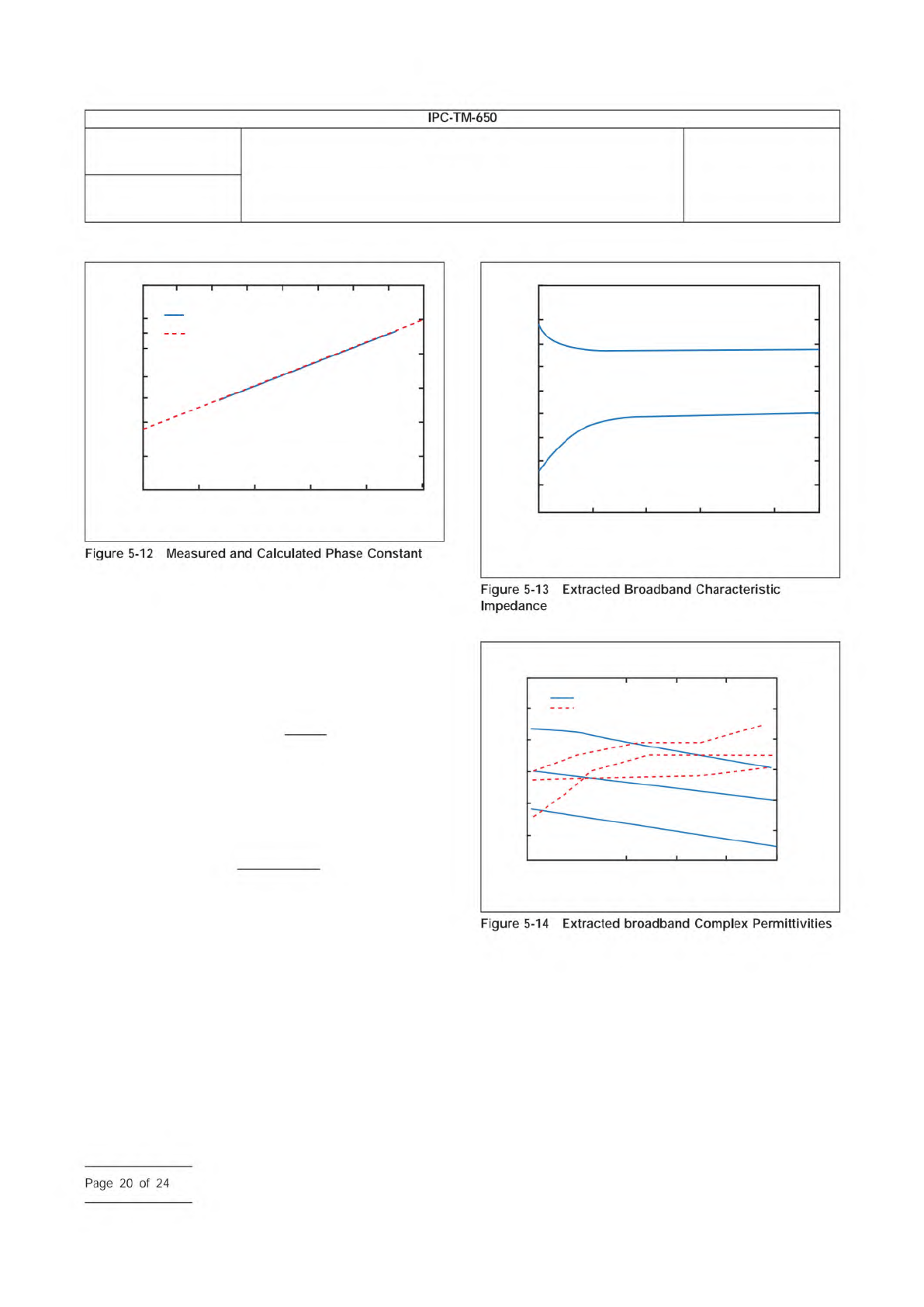
The calculation is iterated until good agreement is obtained.
Agreement is assessed visually. Each time, the high-frequency
values of ε
r
and tanδ are modified. It is recommended to use
a 2D field solver that has a Debye model for the relation
between C and G as described in Equation 5-13 with a large
number of poles to cover a broad frequency range. 30 poles
are considered a good practice.
ε(ω) = ε
∞
+
Σ
i
ε
i
1 + jωτ
i
[5-13]
The solver should be able to smoothly interpolate between the
low frequency values and the high-frequency ones.
The broadband Z
0
(f) is also obtained based on R(f), L(f), C(f),
G(f) as shown in Equation 5-14.
Z
0
=
Γ(ω)
G(ω) + jωC(ω)
[5-14]
An example of such broadband impedance is shown in Figure
5-13.
5.3.6.3.2 Frequency Dependent Complex Permittivity
Extraction
The final R(f), L(f), C(f), and G(f) are used to
extract the complex permittivity using Equation 1-2 and 1-3.
Some examples of extracted permittivities are shown in Figure
5-14.
IPC-25512-5-12
Phase Constant (1/cm)
0.05
0.5
1
2
20
10
5
50
1 2 5 10 20 50
Frequency (GHz)
Measured
Calculated
IPC-25512-5-13
Impedance (Ω)
-80
-60
-40
-20
0
20
40
60
80
100
0.001 0.01 0.1 1 10 50
Frequency (GHz)
Real Zo
Imag Zo
IPC-25512-5-14
Dielectric Constant ε
Dielectic Loss tanδ
3.2
3.4
0.005
0
0.010
0.015
0.020
0.025
0.030
3.6
3.8
2 5
BT
BT
Nelco
Nelco
Nelco
NelcoSI
BT, Nelco 4000–13SI, 6 Layers, 3.75/3.55/3.7
10 20 50
Frequency (GHz)
tan
δ
Number
2.5.5.12
Subject
Test Methods to Determine the Amount of Signal Loss on
Printed Boards
Date
07/12
Revision
A
IPC-TM-650
Figure
5-12
Measured
and
Calculated
Phase
Constant
Figure
5-13
Extracted
Broadband
Characteristic
Impedance
Figure
5-14
Extracted
broadband
Complex
Permittivities
Page
20
of
24
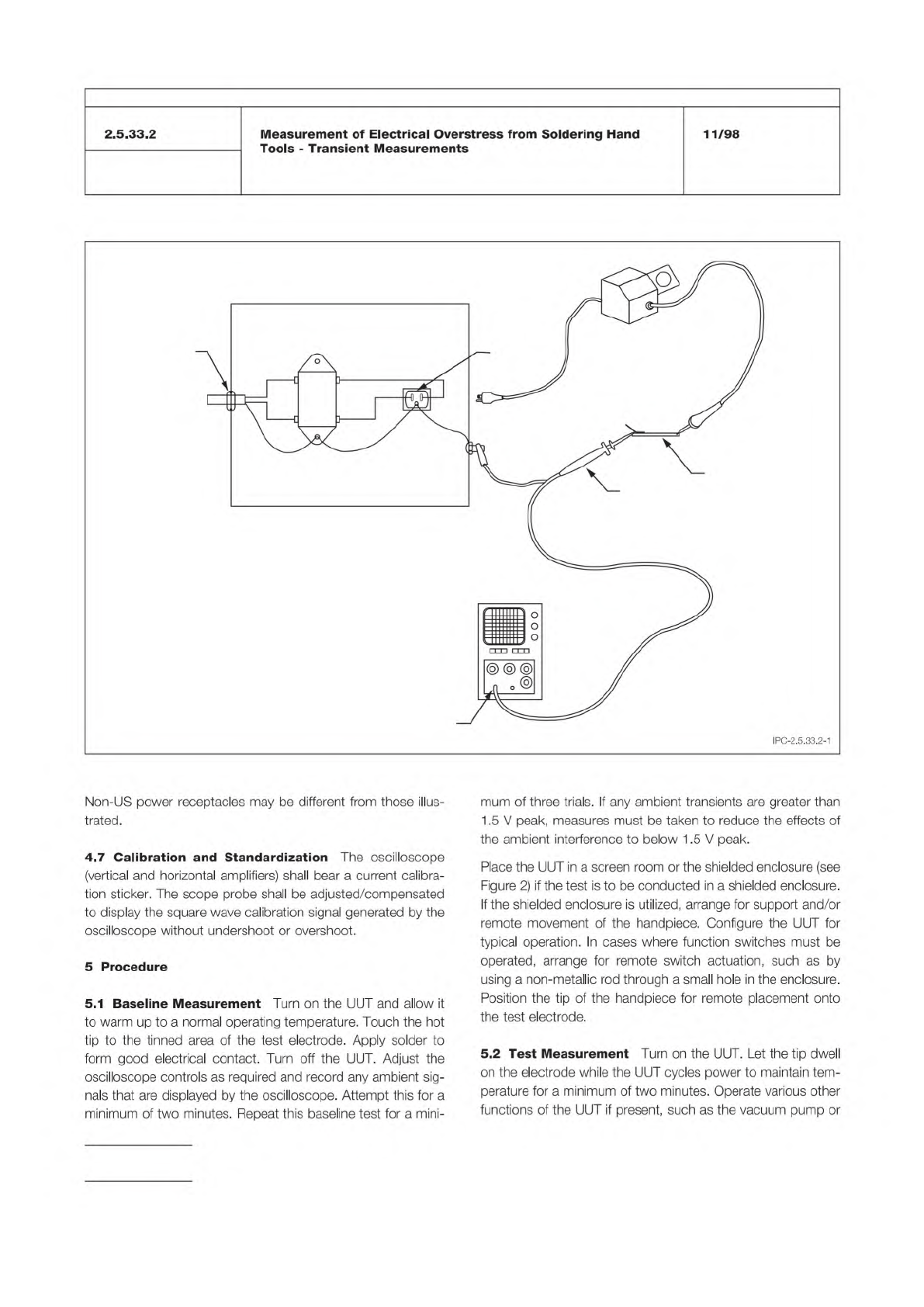
Figure 1 Apparatus for Transient Measurement
OSCILLOSCOPE
AC LINE
FILTER ASSEMBLY
1 MEGOHM
INPUT
RECEPTACLE
FOR UUT
UUT
10 MEGOHM
(X10) SCOPE
PROBE
TEST
ELECTRODE
STRAIN
RELIEF
TO
AC
AC
LINE
FILTER
METAL BOX
BLK BLK
WHTWHT
GRN GRN
G
R
N
IPC-TM-650
Number
Subject Date
Revision
Page 2 of 4
2.5.33.2
Measurement
of
Electrical
Overstress
from
Soldering
Hand
Tools
-
Transient
Measurements
11/98
IPC-2.5.33.2-1
Non-US
power
receptacles
may
be
different
from
those
illus¬
trated.
4.7
Calibration
and
Standardization
The
oscilloscope
(vertical
and
horizontal
amplifiers)
shall
bear
a
current
calibra¬
tion
sticker.
The
scope
probe
shall
be
adjusted/compensated
to
display
the
square
wave
calibration
signal
generated
by
the
oscilloscope
without
undershoot
or
overshoot.
5
Procedure
5.1
Baseline
Measurement
Turn
on
the
UUT
and
allow
it
to
warm
up
to
a
normal
operating
temperature.
Touch
the
hot
tip
to
the
tinned
area
of
the
test
electrode.
Apply
solder
to
form
good
electrical
contact.
Turn
off
the
UUT.
Adjust
the
oscilloscope
controls
as
required
and
record
any
ambient
sig¬
nals
that
are
displayed
by
the
oscilloscope.
Attempt
this
for
a
minimum
of
two
minutes.
Repeat
this
baseline
test
for
a
mini¬
mum
of
three
trials.
If
any
ambient
transients
are
greater
than
1.5
V
peak,
measures
must
be
taken
to
reduce
the
effects
of
the
ambient
interference
to
below
1.5
V
peak.
Place
the
UUT
in
a
screen
room
or
the
shielded
enclosure
(see
Figure
2)
if
the
test
is
to
be
conducted
in
a
shielded
enclosure.
If
the
shielded
enclosure
is
utilized,
arrange
for
support
and/or
remote
movement
of
the
handpiece.
Configure
the
UUT
for
typical
operation.
In
cases
where
function
switches
must
be
operated,
arrange
for
remote
switch
actuation,
such
as
by
using
a
non-metallic
rod
through
a
small
hole
in
the
enclosure.
Position
the
tip
of
the
handpiece
for
remote
placement
onto
the
test
electrode.
5.2
Test
Measurement
Turn
on
the
UUT.
Let
the
tip
dwell
on
the
electrode
while
the
UUT
cycles
power
to
maintain
tem¬
perature
for
a
minimum
of
two
minutes.
Operate
various
other
functions
of
the
UUT
if
present,
such
as
the
vacuum
pump
or