IPC-TM-650 EN 2022 试验方法--.pdf - 第611页
Figure 5 Dual Expo sure Picture TD R Trace Figure 6 T est Cable Hookup IPC-TM-650 Number Subject Date Revision Page 3 of 3 2.5.19 Propagation Delay of Flat Cables Using Time Domain Reflectometer 7/84 A IPC-2-5-19-4 — E F…
Note:
IPC-TM-650
Number
Subject Date
Revision
Page 2 of 3
2.6.23
Test
Procedure
for
Steam
Ager
Temperature
Repeatability
7/93
Each
thermocouple
shall
be
secured
using
positive
mechani¬
cal
means.
For
example,
the
thermocouple
wire
could
be
wound
around
a
piano
wire
secured
across
the
width
of
the
ager.
The
natural
airflow
within
the
ager
should
be
preserved.
Extra
baffles
or
wire
mesh
screens
should
not
be
included
for
this
test,
if
not
used
during
regular
solderability
testing.
Venting
should
be
preserved
as
it
is
during
normal
testing.
The
end
of
the
thermocouple,
including
the
weld
bead
and
exposed
wires,
should
be
oriented
vertically
(pointing
upward)
to
prevent
water
drops
from
collecting
on
them.
5.3
Performing
the
Test
Turn
on
the
ager
and
allow
to
stabilize
until
measurement
procedures
used
during
regular
testing
indicate
stability
has
been
achieved.
Four
hours
is
usually
required
in
most
agers
to
achieve
stability,
and
this
,,warmup^^
time
should
be
included
in
the
production
part
test
procedure.
Start
the
test,
logging
temperature
every
15
minutes
for
8
hours,
(if
the
data
clearly
indicates
that
the
natural
variability
within
the
chamber
varies
more
quickly,
the
sampling
fre¬
quency
can
be
increased
as
necessary)
When
logging
temperatures,
all
thermocouples
should
be
measured
simultaneously,
or
within
2
minutes
maximum.
Temperatures
shall
be
recorded
in
degrees
Celsius.
Measure
temperature
to
the
nearest
0.1
degree.
The
steam
agers
shall
not
be
disturbed
during
the
test,
except
for
routine
maintenance
or
inspection
procedures;
as
used
during
normal
testing.
The
ager
shall
be
tested
without
other
components
inside.
5.4
Test
Conditions
Test
the
temperature
stability
at
the
temperature
set
point
used
for
solderability
testing.
5.5
Data
Analysis
5.5.1
Record
the
following
data
for
each
test.
a.
Ager
manufacturer
and
model
number
b.
Temperature
indicator
type,
date
of
calibration
c.
Test
date
d.
Sampling
frequency
e.
Total
vent
area
on
chamber
lid
[sq.cm]
f.
Total
chamber
cross-sectional
surface
area
[sq.cm]
g.
Total
volume
of
air
in
chamber
[cu.cm]
h.
Set
point
temperature
i.
Test
location
i.
in
hood
ii.
on
table
against
wall
iii.
on
table
in
open
room
j.
Location
of
room
air
conditioning
vents
(include
sketch)
k.
Notes
on
any
special
conditions
during
test
I.
Distance
from
thermocouples
to
water
level
m.
Location
of
thermocouples
inside
ager
(include
sketch)
n.
Room
temperature
when
testing
5.5.2
Test
Data
Prepare
a
matrix
of
test
data,
showing
temperature
of
each
thermocouple
at
each
sampling
interval.
5.5.3
Control
Charts
Prepare
X-bar
and
R
charts
with
appropriate
control
limits.
A
control
limit
calculation
form
is
shown
in
Appendix
1.
Further
instructions
on
preparation
of
control
charts
can
be
found
in
I
PC-
PC-90
or
ANSI/ASQC
Z1.1, Z1.2,
and
Z1.3.
Subgroups
shall
consist
of
all
thermocouples
placed
in
the
ager
(8
or
10),
and
which
are
measured
simultaneously
during
the
test.
The
charts
shall
be
considered
out
of
control
if
any
of
the
fol¬
lowing
applies:
a.
any
one
data
point
is
beyond
the
control
limits
b.
any
2
or
3
consecutive
points
are
near
a
control
limit
(outer
third)
c.
a
run
of
8
or
more
points
is
above
or
below
the
center
line
d.
a
run
of
6
or
more
points
is
increasing
or
decreasing
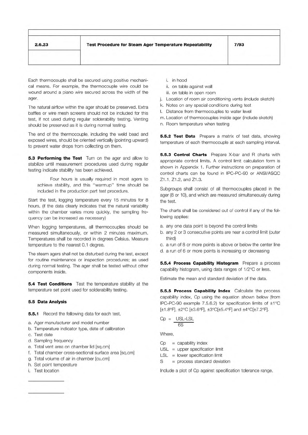
5.5.4
Process
Capability
Histogram
Prepare
a
process
capability
histogram,
using
data
ranges
of
1/2℃
or
less.
Estimate
the
mean
and
standard
deviation
of
the
data.
5.5.5
Process
Capability
Index
Calculate
the
process
capability
index,
Cp
using
the
equation
shown
below
(from
IPC-PC-90
example
7.5.
6.2)
for
specification
limits
of
±1℃
[±1.8°F],
±2℃
[±3.6°F],
±3℃[±5.4°F]
and
±4℃[±7.2°F].
Cp
=
USL-LSL
-
6S
Where,
Cp
二
capability
index
USL
=
upper
specification
limit
LSL
=
lower
specification
limit
S
=
process
standard
deviation
Include
a
plot
of
Cp
against
specification
tolerance
range.
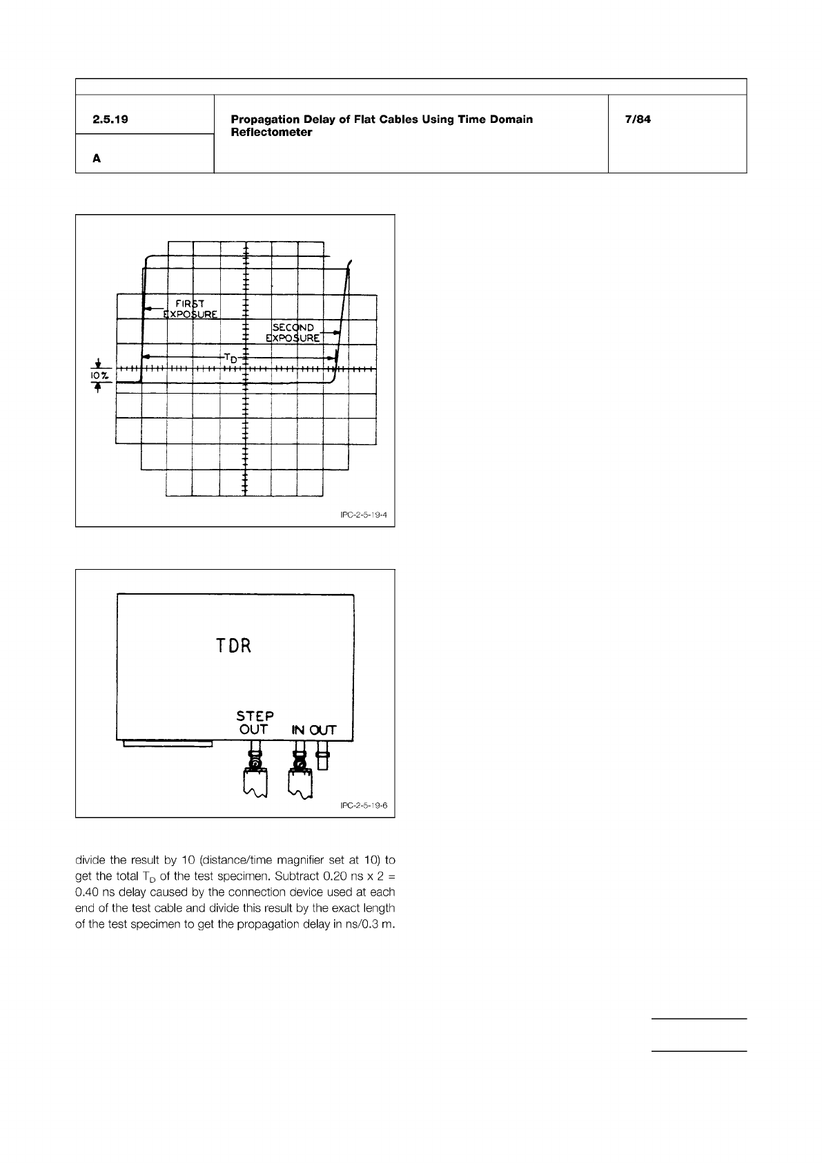
Figure 5 Dual Exposure Picture TDR Trace
Figure 6 Test Cable Hookup
IPC-TM-650
Number
Subject Date
Revision
Page 3 of 3
2.5.19
Propagation
Delay
of
Flat
Cables
Using
Time
Domain
Reflectometer
7/84
A
IPC-2-5-19-4
—
E
FIR
XPQ
ARE
7
:
E
SECC
XPOE
ND
URE”
i
-
i
l
-Tn
・
j
•一一
1111
1
1
1
1
f
>
f
!
”11
t t
t
t
TDR
STEP
OUT
IN
OUT
I
PC-2-5-1
9-6
divide
the
result
by
10
(distance/time
magnifier
set
at
10)
to
get
the
total
TD
of
the
test
specimen.
Subtract
0.20
ns
x
2
=
0.40
ns
delay
caused
by
the
connection
device
used
at
each
end
of
the
test
cable
and
divide
this
result
by
the
exact
length
of
the
test
specimen
to
get
the
propagation
delay
in
ns/0.3
m.
IPC-TM-650
Figure 1 Sample Cable Hanger
The Institute for Interconnecting and Packaging Electronic Circuits
2215 Sanders Road • Northbrook, IL 60062
Material in this Test Methods Manual was voluntarily established by Technical Committees of the IPC. This material is advisory only
and its use or adaptation is entirely voluntary. IPC disclaims all liability of any kind as to the use, application, or adaptation of this
material. Users are also wholly responsible for protecting themselves against all claims or liabilities for patent infringement.
Equipment referenced is for the convenience of the user and does not imply endorsement by the IPC.
Page 1 of 4
IPC-TM-650
TEST
METHODS
MANUAL
1
Scope
This
test
method
describes
the
test
procedures
required
to
measure
propagation
delay
in
flat
cables.
This
test
method
is
an
alternative
to
IPC-TM-650,
Method
2.5.1
9.
Propagation
delay
is
defined
as
the
time
required
for
a
pulse
to
traverse
a
unit
length
of
cable.
Excessive
propagation
delay
will
result
in
the
malfunction
of
critical
circuits
due
to
the
late
arrival
of
pulses.
Propagation
delay
is
directly
proportional
to
the
effective
dielectric
constant
of
the
insulation.
2
Applicable
Documents
Test
Methods
Manual
2
.5.19
Propagation
Delay
of
Flat
Cables
Using
Time
Domain
Reflectometer
(TDR)
3
Test
Specimen
3.1
One
pre-production
or
production
sample
0.9
m
to
3
m
long.
The
number
of
test
samples
should
be
determined
by
the
manufacturer
and/or
user.
4
Equipment/Apparatus
4.1
Oscilloscope:
Tektronix
7623
with
a
7B53A
dual
time
base,
or
equivalent.The
oscilloscope
is
dual
time
based,
trig¬
gered
by
the
pulse
generator,
and
capable
of
accuracy
to
5
ns/div.
4.2
Pulse
generator:
Tektronix
PG501
,
Hewlett-Packard
801
3B,
or
equivalent.
The
pulse
characteristics
from
the
pulse
generator
should
be
determined
by
the
manufacturer
and/or
user.
4.3
Oscilloscope
test
probes,
preferably
high
speed,
with
matched
propagation
delay
4.4
Cable
holder:
Fixture
of
plexiglass
or
other
nonmetallic
material
4.5
Cable
hangers
to
suspend
the
cable
in
air
(see
Figure
1)
4.6
A
termination
resistor
equal
to
the
characteristic
imped¬
ance
of
the
test
specimen
is
required
to
terminate
the
output
end
of
the
cable.
When
oscilloscope
probes
are
attached
to
the
cable,
the
termination
resistance
(RT)
has
to
be
calculated:
Number
2.5.19.1
Subject
Propagation
Delay
of
Flat
Cables
Using
Dual
Trace
Oscilloscope
Date
Revision
7/84
A
Originating
Task
Group
R
_
RpROBE
+
ZoCABLE
RpROBE
-ZqcaBLE
4.7
An
input
resistor
is
required
in
series
between
the
pulse
generator
and
the
test
specimen
(only)
when
the
characteris¬
tic
impedance
of
the
cable
is
equal
to
or
less
than
the
output
impedance
of
the
pulse
generator.
In
this
case:
Input
Resistance
=
ZoGENERATOR
-
ZoCABLE
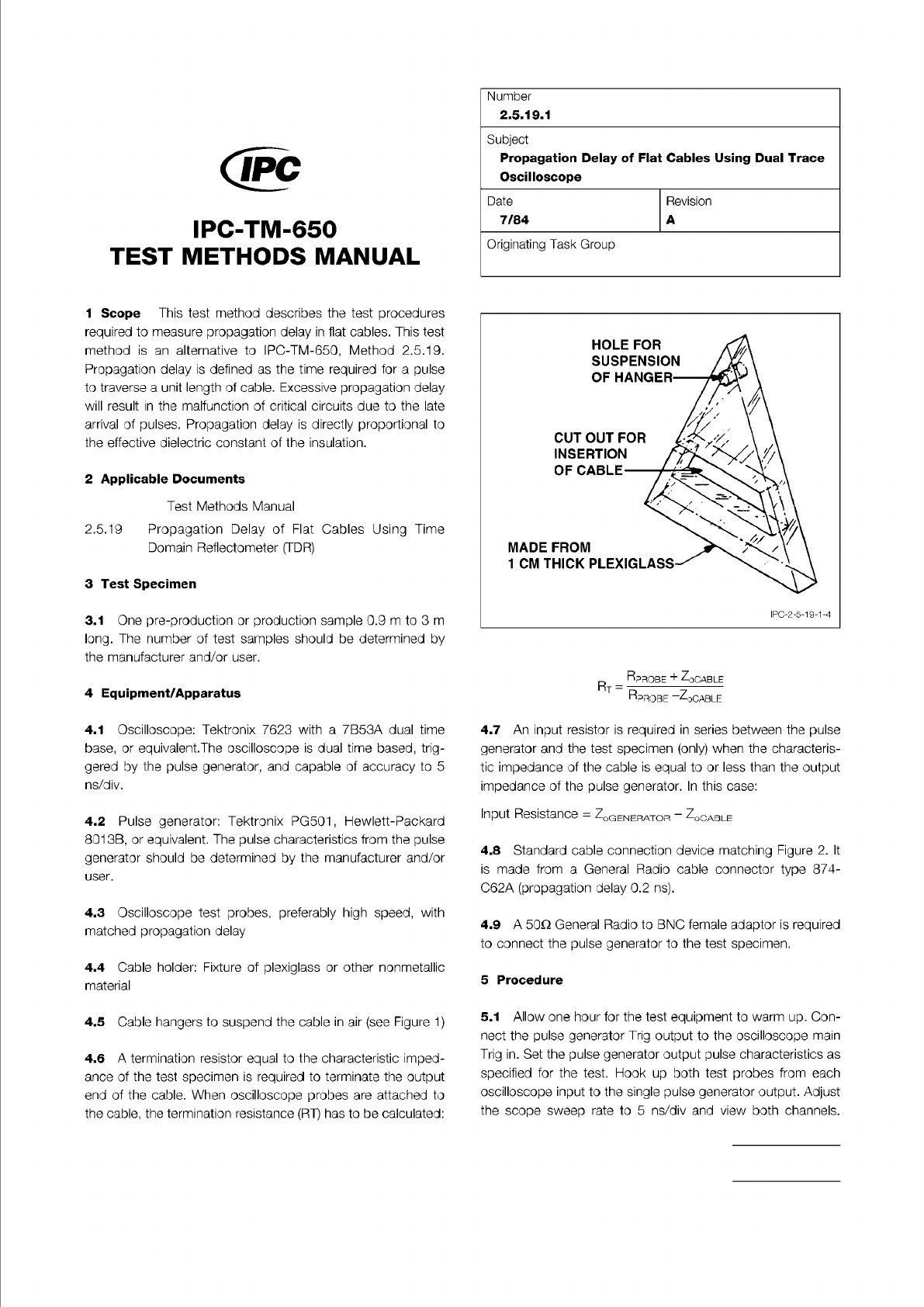
4.8
Standard
cable
connection
device
matching
Figure
2.
It
is
made
from
a
General
Radi。
cable
connector
type
874-
C62A
(propagation
delay
0.2
ns).
4.9
A
50Q
General
Radio
to
BNC
female
adaptor
is
required
to
connect
the
pulse
generator
to
the
test
specimen.
5
Procedure
5.1
Allow
one
hour
for
the
test
equipment
to
warm
up.
Con¬
nect
the
pulse
generator
Trig
output
to
the
oscilloscope
main
Trig
in.
Set
the
pulse
generator
output
pulse
characteristics
as
specified
for
the
test.
Hook
up
both
test
probes
from
each
oscilloscope
input
to
the
single
pulse
generator
output.
Adjust
the
scope
sweep
rate
to
5
ns/div
and
view
both
channels.