Anritsu机器学习应用于PCB外观检测.pdf - 第5页

Anritsu T echnical Review No.28 September 2020 Application of M achine Learni ng to Printed Ci rcuit Board Ex ternal Inspecti on (5) (3) Discrimination Procedure W e used a convolutional neural network with excellent ima…

Anritsu Technical Review No.28 September 2020 Application of Machine Learning to Printed Circuit Board External Inspection

(4)

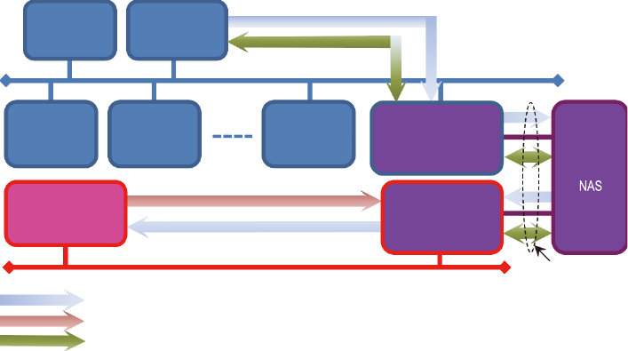
This software was run on one Image Training PC on the

AOI LAN (Figure 4).

AOI-related PCs are connected over a dedicated AOI local

area network (LAN) from the viewpoint of higher security

and to prevent non-factory network problems affecting

plant mass-production.

To assure the independence of the AOI LAN, the ma-

chine-learning environment ( and  in Figure 4) was con-

figured on the in-company LAN via a separate independent

LAN (c. Independent LAN in Figure 4) and multiport Net-

work Attached Storage (NAS) ( in Figure 4).

Required data is shared via files on the NAS and the PC

for capturing learning images is programed to send images

and evaluation data stored on the AOI-DB server periodi-

cally to the machine-learning PC.

Generally, at machine learning, only images of pass

products are required, but not images of faulty products.

However, due to disk-space limitations at the AOI-DB serv-

er, there were problems with inability to save images for

products evaluated as pass. Consequently, the focus of at-

tention was only on trouble locations such as electrodes and

leads for images of parts evaluated as fail and machine

learning was used to capture images of fillets of electrodes

and leads of pass parts from within images of fail parts.

When introducing machine evaluation to external inspec-

tion, the learning model obtained from the Ma-

chine-Learning PC was transferred to the Machine Evalua-

tion PC and the result for the evaluated image was saved in

the AOI-DB server as the visual evaluation result that the

Image Training PC input to the AOI terminal. If images

evaluated by AIO as fail were evaluated by machine learn-

ing as pass, the operator in charge of visual evaluation

handled the image as if it had already been visually evalu-

ated.

Reduction of visual inspection and confirmation by eye is

expected with introduction of machine learning because

only parts evaluated as fail by both AOI and machine

learning are inspected.

5.2 Machine Learning Discriminator

Machine learning is a method for allowing a computer to

learn human-like recognition and evaluation. It is per-

formed using the following two processes: Learning, and

Evaluation

1), 2), 3)

(1) Learning Process

Even the best machine-learning algorithm is worthless

without a learning process which must be performed first

using learning data. Learning is repeated over until the

accuracy (learning mistakes) reach the required accuracy

and the learning model is completed.

(2) Evaluation Process

The discriminator (model with completed learning) eval-

uates whether input image data are pass or fail. For exam-

ple, a discriminator that has learned labelled (named)

product images can accurately evaluate the names of prod-

ucts for unknown images that have not been learned.

a. AOI LAN

b. Company LAN

(1) Training image and AOI evaluation result

(2)

Evaluation m

achine learning model

(3) Board evaluation image and result (at machine evaluation introduction)

(1)

(2)

(3)

(1)

c. Inde

endent LAN

 Image

Training PC

(Windows10)



AOI-DB

Server

AOI

Main

AOI

Terminal

AOI

Terminal

AOI

Terminal

 Machine

Learning PC

(Linux)

 Machine

Evaluation

PC (Linux)

Figure

Image Acquisition System Configuration

Anritsu Technical Review No.28 September 2020 Application of Machine Learning to Printed Circuit Board External Inspection

(5)

(3) Discrimination Procedure

We used a convolutional neural network with excellent

image-recognition performance as the machine-learning

discriminator. A convolutional neural network is configured

from a pile of levels, such as convolution layers and pooling

layers with various special functions to form a number of

deep levels. The convolutional neural netwok used in this

study had 10 levels composed of convoluted layers with co-

efficients of 3 × 3 and 3 × 1 (height × width).

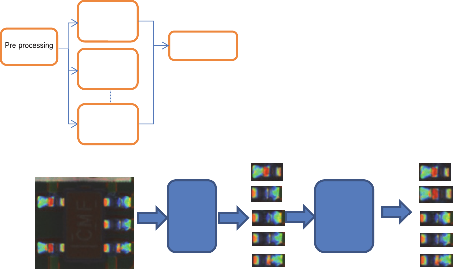
Figure 5 illustrates the discrimination procedure. First,

pre-processing loads the image to be inspected and identi-

fies the solder locations. The solder locations identified by

the discriminator are output as numeric discrimination re-

sults in the range of 0.0 to 1.0 indicating the normality dis-

tribution of the solder locations, with a value of 1.0 being

maximum normality. The normality threshold value deter-

mines whether the solder joint condition is pass or fail.

As shown in Figure 6, this inspection uses multiple dis-

criminators and evaluation is performed using the model

average, which averages the output of each discriminator.

Better performance can be expected

1), 2)

with suppressed

randomness, etc., by changing the learning parameter de-

fault values and combining multiple discriminators than

when using a single discriminator.

Figure 6 Model Averaging

6 Evaluating Results of PC Board External In-

spection using Machine Learning

6.1 Detection Performance

The performance of the algorithm proposed in this article

was evaluated using the model averaging technique applied

to 560 inspection images of pre-specified parts (60 pass

parts and 500 fail parts). The images used for evaluation

were not used for learning.

The results are shown in Table 1; eight learning models

were provided. As shown in Table 1, model averaging was

performed without making a specific evaluation to suppress

randomness in the detection performance for each learning

model.

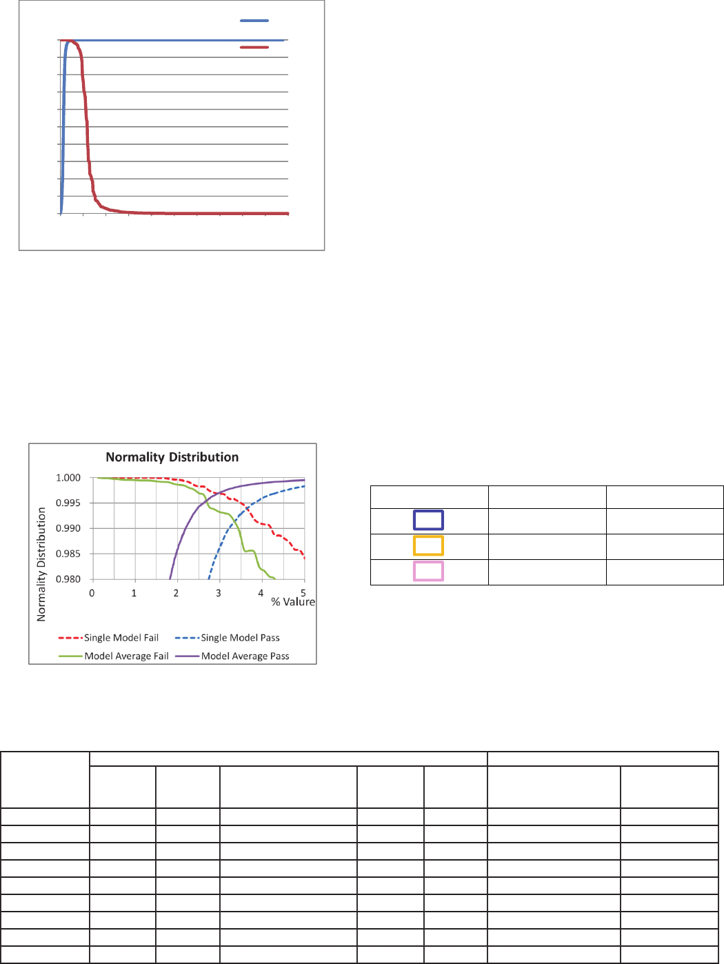
Figure 7 shows the cumulative distribution confirming

the normality distribution. The red line is the cumulative

distribution of normality for fail parts (493 locations) and

the blue line is the cumulative distribution of normality for

pass parts (65,168 locations). The fail parts cumulative dis-

tribution origin is 1.0, but is best if distributed in the lower

half with the origin at less than 0.5. In addition, the pass

parts cumulative distribution is the distribution with 0.0 as

the origin, but is best if distributed in the upper half with

the origin at more than 0.5. Since the cumulative distribu-

tions for the pass and fail locations intersect, evaluation

mistakes occur when evaluating using a threshold.

Machine

Learning

Discriminator 1

Machine

Learning

Discriminator 2

Model Average

Machine

Learning

Discriminator N

Machine

Learning

Discriminator

Inspection

Image

(Input Image)

Extraction of Slder

Joints at 5 Locations

Discrimination

Processing for Each

Location

Normality of Each

Joint

Pre-

processing

0.2

0.3

0.8

0.9

1.0

Figure 5 Discrimination Procedure using Machine Learning

Anritsu Technical Review No.28 September 2020 Application of Machine Learning to Printed Circuit Board External Inspection

(6)

Figure 7 Normal Board Distribution

Figure 8 shows a comparison of the normality for the

model average and single model results. The value for pass

locations increases by using the model average compared to

not using it, and the normality improves because the value

for fail locations decreases. However, evaluation mistakes

occur when using the evaluation threshold due to the dis-

tribution intersection.

Figure 8 Comparison of Model Average and Single Model

Normal Board Distribution

6.2 Distribution of Board Image Evaluation Mis-

takes

To confirm the mis-detection phenomenon, actual images

were checked. Figures 9 to 11 show examples of fail results

using machine learning. For AOI-evaluated fault locations,

on-site visual inspections were performed by a specialist

and the results were compared with the machine-learning

results. In these figures, locations evaluated as pass by AOI

are enclosed in a blue frame, while those evaluated by AOI

as fail are enclosed in an orange frame; locations evaluated

as fail by both AOI and visual inspection are enclosed in a

pink frame. The numerical values in Figures 10 and 11 in-

dicate the normality output by machine learning. The or-

ange-frame locations in Figure 10 were evaluated as fail by

AOI but pass by visual inspection. We clearly see the high

numeric value of the results assigned by machine learning

to these orange locations. Additionally, the pink frames in

Figure 11 which were evaluated as fail locations by both

AOI and visual inspection, were assigned low numeric val-

ues by machine learning. The machine-learning normality

output is extremely close to the results of visual evaluation

by a specialist.

Frame Color AOI Evaluation Visual Evaluation

Pass ―

Fail Pass

Fail Fail

Figure 9 Classification Method

0.1

0.2

0.3

0.4

0.5

0.6

0.7

0.8

0.9

10%

20%

30%

40%

50%

60%

70%

80%

90%

100%

Normality Distribution

見過ぎ(10)

実不良(11)

Pass

Fail

Table 1 Detection Performance

Training Model

500 Images (Failure) 60 Images (Pass)

Failure Pass

Number of

Miss-Fail Detection

Detection

Ratio

Miss-

Detection

Number of

Fail-Detection at Excess

Watching

Reduction Ratio

of Fail Detection

1 545 495 50 0.91 28 0 0.00

2 545 504 41 0.92 25 0 0.00

3 545 478 67 0.88 11 0 0.00

4 545 497 48 0.91 17 3 0.04

5 545 496 49 0.91 20 0 0.00

6 545 495 50 0.91 10 4 0.06

7 545 489 56 0.90 21 0 0.00

8 545 501 44 0.92 26 3 0.04

Model Average 545 495 50 0.91 12 0 0.00