s26030829.pdf - 第11页
Sensors 2026 , 26 , 829 11 of 21 (2) Establish the relationship between t 1 , t 2 , and total time t 3 , and use the central dif- ference method to derive the acceleration of the for earm. Construct an energy cost functi…
Sensors 2026, 26, 829
10 of 21
(a) (b)
(c) (d)
(e) (f)
(g) (h)
Iteration#
F4
PSO
MOGGO
GWO
WOA
NSGAII
DBO
Iteration#
F5
PSO
MOGGO
GWO
WOA
NSGAII
DBO
Iteration#
F9
PSO
MOGGO
GWO
WOA
NSGAII
DBO
Iteration#
F15
PSO
MOGGO
GWO
WOA
NSGAII
DBO
Iteration#
F21
PSO
MOGGO
GWO
WOA
NSGAII
DBO
Iteration#
F23
PSO
MOGGO
GWO
WOA
NSGAII
DBO
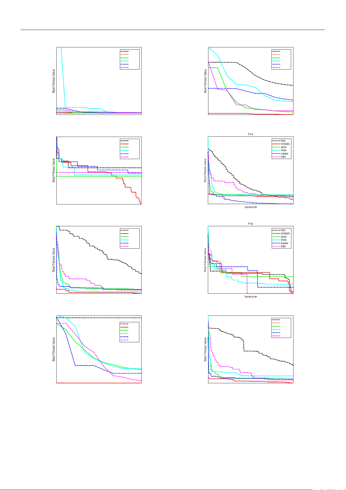
Figure 4. Convergence Curves for a Subset of the CEC2013 Test Functions.
It is triggered when an individual does not satisfy the condition t
1
< t
2
< t
3
, and is
randomly assigned a larger value to make the individual enter the exploration group to
perform a deep search.
https://doi.org/10.3390/s26030829
Sensors 2026, 26, 829
11 of 21
(2) Establish the relationship between t
1
, t
2
, and total time t
3
, and use the central dif-
ference method to derive the acceleration of the forearm. Construct an energy cost function.
By combining this function with the displacement equation and assigning weight values, a
composite multi-objective function is obtained. Through global search by the exploration
group and local optimization by the utilization group, the current optimal solution is
determined. If the maximum preset number of iterations is reached, the iteration stops.
(3) Using the proposed GGO-based optimization under the prescribed constraints,
the optimal switching times t
1
and t
2
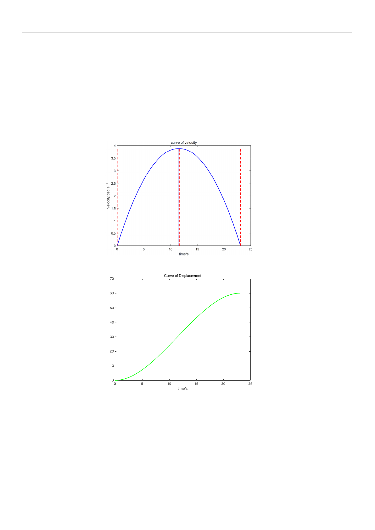
were determined. The resulting kinematic profiles
(velocity, displacement, acceleration, and jerk versus time) were then generated in MATLAB
for subsequent analysis, as presented in Figures 5–7.
Figure 5. Velocity trajectory planning profile.
Position/deg
Figure 6. Displacement–time trajectory profile.
The simulation results indicate that the proposed polynomial interpolation–based
trajectory planning method enables the manipulator’s angular velocity to vary continu-
ously and smoothly throughout the entire motion. This significantly mitigates mechanical
vibration and impact induced by abrupt velocity variations, thereby helping to reduce os-
cillations of the end-effector. Moreover, the method imposes a lower computational burden
on the control system, and the acceleration variation can be interpreted more intuitively
substituting the optimal solution t
3
into the energy cost function, the optimal vibration
energy index under the prescribed weight constraint can be obtained. The double-parabola–
trapezoidal velocity planning profile derived from the Graylag Goose Optimization (GGO)
https://doi.org/10.3390/s26030829
Sensors 2026, 26, 829
12 of 21
parameters is shown in Figure 5. Overall, the profile is relatively smooth, with no abrupt
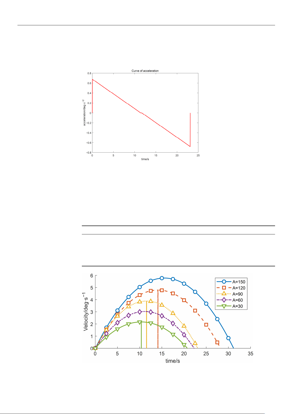
changes in velocity. Moreover, as indicated by the displacement curve in Figure 6 and
the acceleration curve in Figure 7, the angular variation is gradual, and the acceleration
exhibits no pronounced fluctuations.
Figure 7. Acceleration–time profile.
5. Comparison Under Different Initial Input Conditions
(1) By modifying the motion range of the wafer-transfer manipulator, i.e., varying the
angular displacement A, the corresponding trajectories and the residual vibration energy
can be rapidly fitted through iterative computation. With all other conditions unchanged,
the experimental results are summarized in Table 5 and Figures 8–10.
Table 5. Variation in Objective Function Values of Wafer Transfer Robot Arm at Different Displacements.
Displacement Runtime Vibration Energy Index E
vib
150 16.8 347.8261
120 13.8 347.8261
90 9.633 339.394
60 7.083 166.957
30 6.033 164.882
Figure 8. Velocity-time profiles for different planned displacements.
https://doi.org/10.3390/s26030829