s26030829.pdf - 第5页
Sensors 2026 , 26 , 829 5 of 21 Then the total kinetic energy of the r obotic arm is: T = T 1 + T 2 = 1 2 m 1 v 2 c 1 + 1 2 I 1 . q 2 1 + 1 2 m 2 v 2 c 2 + 1 2 I 2 ( . q 1 + . q 2 ) 2 (2) I 1 and I 2 repr esent the momen…
Sensors 2026, 26, 829
4 of 21
defined by the DH parameters, whereas
θ
represents the elastic deformation angle of the
flexible transmission element.
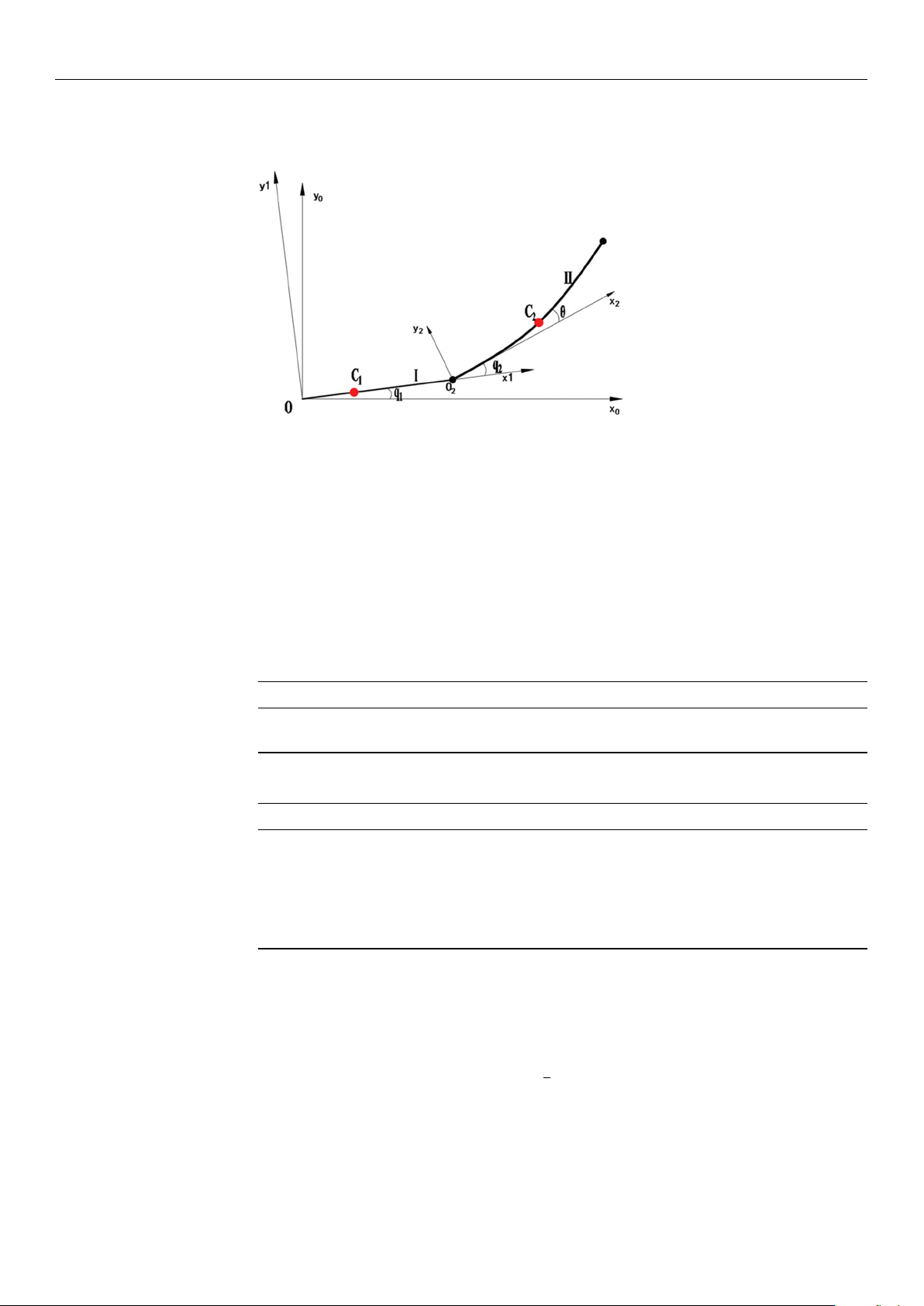
Figure 1. Motion Model of Wafer Transport Robotic Arm.
Table 1 shows the simplified model of the wafer transport robot, which consists of the
rigid link I (upper arm) and the flexible link II (lower arm). The world coordinate system
X
0
OY
0
is established with the base as the origin, the coordinate system X
1
OY
1
is set at the
end-point of link I (upper arm), and the coordinate system X
2
O
2
Y
2
is established at the
end-point of link II (lower arm). C
1
and C
2
represent the center of mass of the two links.
q
1
is the rotation angle of the primary arm, q
2
is the rotation angle of the secondary arm,
and
θ
is the deformation of the flexible lower arm. The structural parameters of the wafer
transfer robotic arm in this study are shown in Table 2.
Table 1. D-H Parameter Table of the Wafer Handling Robot Arm.
Arm/li q
i
/
◦
d
i
/mm l
i
/mm α
i
/
◦
L
1
0–120 0 240 0
L
2
0–120 0 240 0
Table 2. Parameters of Components of the Wafer Transport Robotic Arm.
Structure Value
Primary arm length/L
1
240 mm
Secondary arm length/L
2
240 mm
Mass of Primary arm/m
1
2.757 kg
Mass of secondary arm/m
2
2.165 kg
The center of gravity of the primary arm/Lc
1
0.4 L
1
The center of gravity of the secondary arm/Lc1 0.5 L
2
First, based on the Lagrange method, the dynamic equations of a planar two-degree-of-
freedom rigid robot are established. First, the robot’s potential energy equation is analyzed.
The robot’s forearm can be regarded as a flexible arm rod, and its elastic potential energy
can be expressed as
V
e
=
1
2
k(q
2
− θ
2
) (1)
Here, the
θ
refers to the ideal angle of the forearm when no deformation occurs. Since
the robot prototype moves parallel to the ground throughout, gravitational potential energy
is not taken into account. The kinetic energy expression includes both the rotational kinetic
energy of each link and the translational kinetic energy of the link centers of mass.
https://doi.org/10.3390/s26030829

Sensors 2026, 26, 829
5 of 21
Then the total kinetic energy of the robotic arm is:
T = T
1
+ T
2
=
1
2
m
1
v
2
c1
+
1
2
I
1
.
q
2
1
+
1
2
m
2
v
2
c2
+
1
2
I
2
(
.
q
1
+
.
q
2
)
2
(2)
I
1
and I
2
represent the moments of inertia of the link about its center of mass. Since
both the upper arm and forearm rotate around their joints, the moments of inertia of the
upper arm and forearm are:
I
1
=
1
3
m
1
l
2
1
, I
2
=
1
3
m
2
l
2
2
(3)
The Lagrange function of the robotic arm is:
L = T − V =
1
2
(I
1
+ m
2
l
2
1
+ I
2
)
.
θ
2
1
+
1
2
I
2
.
θ
2
2
+ I
2
.
θ
1
.
θ
2
+ m
2
l
1
l
c2
.
θ
1
(
.
θ
1
+
.
θ
2
) cos θ
2
−
1
2
k(θ
2
− θ
o
)
2
(4)
Based on the Lagrange function, the Lagrange equations are further applied to each
generalized coordinate.
The Lagrange dynamic equation of the lower arm is:
d
dt
∂L
∂
.
q
1
!
−
∂L
∂q
1
= τ
1
(5)
The Lagrange dynamic equation of the upper arm is:
d
dt
∂L
∂
.
q
2
!
−
∂L
∂q
2
= τ
2
(6)
The dynamic model of the wafer transfer robot system is:
"
τ
1
τ
2
#
=
"
M
11
M
12
M
21
M
22
#"
..
q
1
..
q
2
#
+
"
C
11
C
12
C
12
C
22
#"
.
q
1
.
q
2
#
+
"
0
k(q
2
− θ)
#
(7)
In Equation (7), the stiffness term k(q
2
− θ
) represents the restoring torque induced
by the elastic deformation of the flexible transmission and is applied to the corresponding
joint equation.
3. Vibration Suppression Trajectory Planning for Robotic Arms Based on
Graylag Goose Algorithm
Existing robot trajectory planning methods include cubic and quintic polynomial
trajectory planning algorithms [
32
–
34
], T-shaped and S-shaped acceleration-deceleration
trajectory planning algorithms, and B-spline trajectory planning algorithms. During the
operation of a wafer handling manipulator, the start and end positions are known, while
the motion states during the process are unknown. This study uses a cubic polynomial
interpolation method to plan the motion trajectory [
35
]. This method combines the low
impact and high stability of S-shaped trajectory planning with the low computational
load of T-curve planning. It is easy to program and debug, has high reliability, and can
avoid sudden changes in acceleration, thereby effectively suppressing vibrations at the
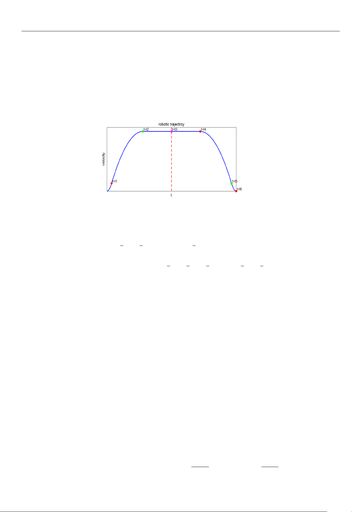
manipulator’s end. As shown in Figure 2, the polynomial trapezoidal interpolation curve
trajectory is defined over the interval (0, t
6
). The robotic arm first experiences smooth
startup acceleration, the acceleration decreases beginning at time t
1
, and reaches constant
https://doi.org/10.3390/s26030829
Sensors 2026, 26, 829
6 of 21
velocity at time t
2
. If t = t
4
, the speed begins to decelerate until it reaches 0 at t
6
, achieving a
smooth stop. The trajectory expression is given in Equation (8).
.
q =
at
2
, 0 < t < t
1
bt
2
+ ct + d, t
1
< t < t
2
bt
2
2
+ ct
2
+ d, t
2
< t < t
4
b
′
t
2
+ c
′
t + d
′
, t
4
< t < t
5
a(t − 2t
3
)
2
, t
5
< t < t
6
(8)
Figure 2. Velocity planning S-shaped curve.
Let the angular displacement of the wafer transport robotic arm be A, then its dis-
placement equation can be expressed in Equation (9).
2
3
at
3
1
+
2
3
bt
3
2
+ ct
2
2
+ 2dt
2
−
2
3
bt
3
1
− ct
2
1
− 2dt
1
+ 2(t
3
− t
2
)(bt
2
2
+ ct
2
+ d) = A (9)
P =
1
3
at
3
1
+
1
3
bt
3
2
+
1
2
ct
2
2
+ dt
2
−
1
3
bt
3
1
−
1
2
ct
2
1
− dt
1
(10)
Q = bt
2
2
+ ct
2
+ d (11)
For the convenience of deriving the formula, we replace part of the polynomial in the
displacement formula with P and Q, as shown in Equations (10) and (11).
The rate of change in jerk directly affects the efficiency of these energy losses, espe-
cially during the initial impact or rapid change stages. In a vibration system, the integral
over time of the square of the jerk reflects the residual vibration energy of the system
during rapid start-stop processes. To quantitatively evaluate vibration suppression per-
formance, Equation (12) defines the residual vibration energy as the time integral of the
squared jerk. Since jerk represents the rate of change in acceleration, minimizing this index
effectively suppresses high-frequency excitation and residual oscillations during rapid
start–stop motions.
In this study, the planned velocity profile is designed to be symmetric with respect
to the mid-time instant t
3
. As a result, the jerk-related vibration energy contributed by
the second half of the motion [t
3
, t
6
] is identical to that of the first half [t
0
, t
3
]. Therefore,
for conciseness, Equation (12) evaluates the vibration energy over [t
0
, t
3
], and the total
vibration energy over the complete motion interval [t
0
, t
6
] can be obtained.
E
vib
=
Z
t
3
0
(
...
q (t))
2
dt (12)
The multi-objective optimization function is:
Min
(
F(t
1
, t
2
) = ω
1
t
2
+
30 − P
Q
+ ω
2
"
4a
2
t
1
+ 4
at
1
t
1
− t
2
2
(t
2
− t
1
)
#)
(13)
https://doi.org/10.3390/s26030829