s26030829.pdf - 第8页
Sensors 2026 , 26 , 829 8 of 21 If the maximum number of iterations is reached, it is consider ed that the final solution has been achieved, and the iteration stops, exporting the current optimal solution. And its logical…

Sensors 2026, 26, 829
7 of 21
Optimization is the process of finding the best solution to a problem among all possible
alternatives [
36
–
38
]. The Graylag Goose Optimization (GGO) algorithm, as an emerging
metaheuristic algorithm, is inspired by the intelligent behaviors of gray geese during long-
distance migration, such as efficient formation flying, cooperative resting, and dynamic
leadership. The algorithm simulates mechanisms like “leader goose switching,” “flock
following,” and “energy conservation,” enabling a finer balance between convergence
accuracy and optimization speed.
The Graylag Goose Optimization (GGO) algorithm consists of two stages: global
exploration and local optimization. Based on the constraints of the objective function,
a fitness function is defined. After setting the population size, all randomly generated
individuals enter the initial exploration group. The population is then sorted according to
fitness values, and the top N solutions in terms of fitness are defined as the exploitation
group, while the remaining poorer solutions form the exploration group. Individuals that
meet the fitness function criteria are assigned to the “exploitation group,” whereas those
that do not are given high penalty values and re-enter the exploration group to search for
solutions. The initial parameters of the population are shown in Table 3.
Table 3. Origin Parameter of graylag goose population.
Parameter Value
Population size/N 50
Maximum number of iterations/M 200
Minimum time interval/δ 0.1
First, randomly generate N arbitrary solutions. The individual position update strategy
of the Graylag Goose Optimization Algorithm is divided into two parts: global search by
the exploration group and local optimization by the exploitation group. If an individual’s
value does not meet the requirements of the fitness function, assign a high penalty value to
that individual.
Explore group global search:
Strategy 1: Move toward the global best solution X
best
.
x
new
= x
best
− A ·
|
C · x
best
− x
|
(14)
A = 2
(
1 − iter/MaxIter
)
· r
1
+ (1 − iter/MaxIter), C = 2r
2
(15)
The r
1
and r
2
is random Vector
Strategy 2: Guided by Three Random Geese.
x
new
= ω
1
x
r1
+ zω
2
(x
r2
− x
r3
) + (1 − z)ω
3
(
x − x
r1
)
(16)
Partial optimization by the development team
Strategy 1: The three-sentinel geese seek the average value, where the sentinel geese
individuals are selected from the three best solutions in the group based on fitness.
x
new
=
1
3
(
x
s1
+ x
s2
+ x
s3
)
(17)
Strategy 2: Perturbation Near the Current Optimal Solution.
x
new
= x + 0.5(1 + z)ω(x − x
best
) (18)
https://doi.org/10.3390/s26030829
Sensors 2026, 26, 829
8 of 21
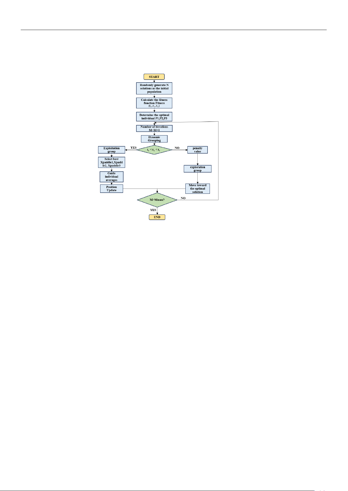
If the maximum number of iterations is reached, it is considered that the final solution
has been achieved, and the iteration stops, exporting the current optimal solution. And its
logical sequence diagram is shown in Figure 3.
Figure 3. Logical Flowchart of the Graylag Goose Optimization Algorithm.
4. Algorithm Testing and Analysis
To verify the performance of the multi-objective GGO function in different workspaces,
five metaheuristic optimization algorithms—Particle Swarm Optimization (PSO) [
14
], Gray
Wolf Optimizer (GWO) [
18
], Whale Optimization Algorithm (WOA) [
26
], Non-dominated
Sorting Genetic Algorithm II (NSGAII) [
10
], and Dung Beetle Optimization (DBO) [
23
]—
were added on the MATLAB 2022B platform for comparison with the multi-objective
GGO function. Two unimodal functions, four multimodal functions, and two composite
functions from the CEC2013 benchmark test set were selected as objective functions, as
shown in Table 4. The performance of the multi-objective GGO algorithm was evaluated
by comparing the results of the test set runs.
In Table 4, a subset of benchmark functions from the CEC2013 test suite is selected to
evaluate the optimization performance of the proposed algorithm. Specifically, functions
F4 and F5 are representative unimodal functions used to assess exploitation capability and
convergence accuracy, whereas F9, F14, F15, F16, F21, and F23 are multimodal or composite
functions designed to evaluate global search ability and robustness against local optima.
These functions cover different landscape characteristics, including high dimensional-
ity, strong nonlinearity, and multiple local minima, which are consistent with the complexity
of multi-objective trajectory optimization problems in robotic systems.
Based on the original Gray Goose Optimization (GGO) algorithm, this study further
develops an improved multi-objective variant to better address the dual-objective vibration
suppression trajectory optimization problem.
https://doi.org/10.3390/s26030829

Sensors 2026, 26, 829
9 of 21
Table 4. CEC Function Test Results.
Function PSO NSGAII GWO WOA DBO MOGGO
F4
Mean
1.83 × 10
8
9.87 × 10
6
1.30 × 10
7
4.23 × 10
7
3.02 × 10
8
6.62 × 10
4
Std
6.78 × 10
8
9.83 × 10
6
7.06 × 10
7
9.44 × 10
7
2.10 × 10
8
3.91 × 10
4
F5
Mean
3.78 × 10
7
1.62 × 10
6
3.37 × 10
6
7.36 × 10
5
1.06 × 10
5
8.5 × 10
3
Std
5.25 × 10
7
7.19 × 10
6
4.56 × 10
6
6.15 × 10
6
2.12 × 10
6
9.47 × 10
3
F9
Mean −557.91 −557.61 −556.16 −556.8 −557.27 −558.48
Std 2.6599 1.8035 2.2561 1.8668 1.8109 3.6466
F14
Mean
1.97 × 10
4
1.11 × 10
3
9.82 × 10
3
9.93 × 10
3
7.41 × 10
3
7.95 × 10
3
Std
1.25 × 10
4
4.59 × 10
3
3.28 × 10
3
3.16 × 10
3
4.12 × 10
3
871.7893
F15
Mean
2.05 × 10
4
1.24 × 10
4
9.4 × 10
3
8.76 × 10
3
9.21 × 10
3
7.35 × 10
3
Std
1.13 × 10
4
4.50 × 10
3
2.52 × 10
3
3.12 × 10
3
2.26 × 10
3
1.08 × 10
3
F16
Mean 204.0242 203.6665 203.8356 204.1670 203.9555 203.9054
Std 0.6995 0.3577 0.3197 0.3353 0.4455 1.3284
F21
Mean
7.54 × 10
5
1.38 × 10
5
4.06 × 10
4
5.70 × 10
5
8.94 × 10
4
2.98 × 10
3
Std
7.43 × 10
5
3.44 × 10
5
2.18 × 10
5
2.52 × 10
5
2.76 × 10
5
249.0022
F23
Mean
2.14 × 10
4
1.24 × 10
4
1.09 × 10
4
1.09 × 10
4
1.09 × 10
4
9.63 × 10
3
Std
1.26 × 10
4
4.13 × 10
3
2.91 × 10
3
2.37 × 10
3
1.96 × 10
3
819.0361
It should be noted that the proposed Multi-Objective Gray Goose Optimization
(MOGGO) algorithm is an improved version of the original GGO algorithm. In this study, a
Logistic chaotic map is introduced to enhance the diversity of the initial population, while a
Gaussian (normal) disturbance mechanism is incorporated during the optimization process
to improve global exploration ability and avoid premature convergence. In addition, the
original single-objective GGO framework is extended to handle multi-objective optimiza-
tion, making it suitable for solving the dual-objective vibration suppression trajectory
planning problem. The results of the CEC2013 test set are shown in Figure 4. The results
indicate that MOGGO performs the best overall on the CEC2013 test functions, significantly
outperforming the comparison algorithms in terms of convergence speed, solution accuracy,
and stability.
As shown in Figure 4a–h, the convergence behaviors of different algorithms are
compared on benchmark functions F4, F5, F9, F14, F15, F16, F21, and F23. Overall, MOGGO
demonstrates faster convergence speed and better solution accuracy across most test
functions. In unimodal functions, the MOGGO rapidly reaches the optimal region, while in
multimodal and complex functions, it maintains stable convergence and effectively avoids
premature stagnation. In contrast, PSO, WOA, GWO, and NSGA-II generally exhibit
slower convergence or are more prone to local optima. These results indicate that MOGGO
achieves a better balance between global exploration and local exploitation.
(1) Set the forearm to rotate 120
◦
, with the motor’s starting acceleration at 20 deg/s
2
.
On the MATLAB platform, set the population size and number of iterations, define the
main loop function of the algorithm and the displacement equation, and establish it as a
fitness function according to the strict constraint t
1
< t
2
< t
3
. The fitness function can be
expressed as:
F = ω
1
t
3
+ ω
2
E
vib
+ ε (19)
Among them,
1
and
2
are the target weight values, and e is the penalty value. In Equa-
tion (19), w1 and w2 denote the weighting coefficients for motion time and residual vibration
energy, respectively, satisfying w
1
+ w
2
= 1. These parameters allow flexible trade-offs be-
tween efficiency and vibration suppression according to different operational requirements.
https://doi.org/10.3390/s26030829