s26030829.pdf - 第4页
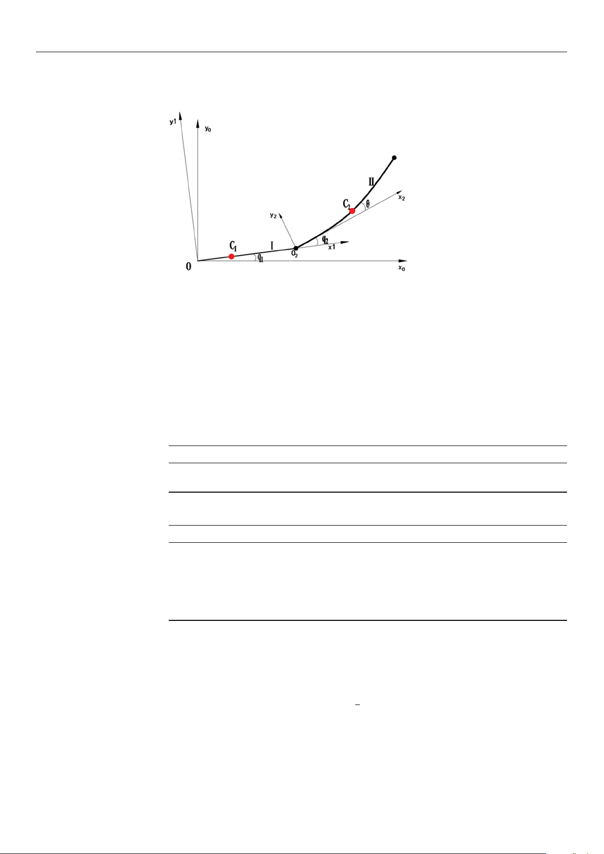
Sensors 2026 , 26 , 829 4 of 21 defined by the DH parameters, wher eas θ repr esents the elastic deformation angle of the flexible transmission element. Figure 1. Motion Model of W afer T ransport Robotic Arm. T able 1 sho…

Sensors 2026, 26, 829
3 of 21
the influence of random disturbances [
15
–
17
]. Researchers have proposed various new
optimization algorithms and introduced different solution strategies to address the short-
comings of these two algorithms. Yue et al. applied a gray wolf optimization algorithm with
a probabilistic disturbance strategy to solve the time-optimal problem. This optimization
strategy effectively balanced the weight between local optimization and global search [
18
].
However, the gray wolf population may converge around suboptimal individuals, leading
to premature convergence issues [
19
,
20
]. Pu Q et al. introduced an improved wild dog
optimization algorithm for robotic arm time-impact optimization [
21
,
22
], but they did not
perform tests for solving high-dimensional problems using the wild dog optimization
algorithm. Additionally, to improve global search capability and address the issue of search
direction disturbance, Lv Yun peng et al. proposed an inverse kinematics solver based on
a multi-strategy improved dung beetle optimization algorithm. However, this improved
algorithm has not been applied to the multi-objective vibration optimization direction [
23
].
Widyianto Agus et al. addressed the issue of the shipboard two-degree-of-freedom robotic
arm being affected by environmental factors and proposed a real-time tuning of PD con-
trol parameters based on an ant colony algorithm, significantly improving the stability of
shipboard equipment [
24
]. Abro et al. combined ant colony optimization’s pheromone
learning with the Denavit–Hartenberg (DH) method to develop a robotic arm error model,
further enhancing the accuracy of global search and improving the reliability and accuracy
of industrial robotic systems [
25
]. However, the ant colony algorithm is heavily depen-
dent on the initial model, making it difficult to avoid local optimal solutions. The Whale
Optimization Algorithm (WOA) introduced a random spiral search step, eliminating the
need for crossover and mutation operators, with a simpler program structure. Wang Fang
et al. applied a hybrid whale optimization algorithm to optimize the time-impact optimal
trajectory of industrial robotic arms, using fifth-order B-splines for interpolation planning
of motion trajectories in joint space [
26
]. However, the performance of this algorithm signif-
icantly deteriorates in a multi-constraint environment and requires further integration with
various improvement strategies [
27
]. The Graylag Goose Optimization (GGO) algorithm
introduced a group migration strategy [
28
], demonstrating strong search capabilities in
multi-objective problems and efficient local optimization when facing suboptimal solu-
tions. Ashish Sharma et al. conducted eight multi-objective benchmark tests, with the
results showing that the Multi-Objective Graylag Goose Optimization (MOGGO) algorithm
exhibited excellent performance in terms of convergence [29].
In summary, this paper introduces the GGO algorithm into the vibration suppression
trajectory optimization problem of wafer transport robotic arms, providing a new feasible
solution for multi-objective trajectory optimization. This study constructs the end dynamics
equation of the flexible lower arm and integrates a multi-objective optimization model
involving motion time, energy, and impact. Based on the multi-objective GGO algorithm,
the trajectory parameters are solved, aiming to generate a set of Pareto-optimal trajectories
with superior overall performance, offering a novel and efficient solution to improve the
performance of the wafer transport system.
2. Establishment of the Dynamics Model for Wafer Transport
Robotic Arm
In this study, the wafer transport robotic arm mainly consists of two links [
30
,
31
]. The
upper (first) link is rigidly connected to the motor, while the lower (second) link is driven
by another motor via a flexible steel belt inside the upper link, which can be regarded as a
flexible motion joint. During motion, only the bending stress of the steel belt is considered.
The end-effector is coupled to the posture of the upper link through the steel belt embedded
inside the lower link. As shown in Figure 1, q1 and q2 denote the rotational joint angles
https://doi.org/10.3390/s26030829
Sensors 2026, 26, 829
4 of 21
defined by the DH parameters, whereas
θ
represents the elastic deformation angle of the
flexible transmission element.
Figure 1. Motion Model of Wafer Transport Robotic Arm.
Table 1 shows the simplified model of the wafer transport robot, which consists of the
rigid link I (upper arm) and the flexible link II (lower arm). The world coordinate system
X
0
OY
0
is established with the base as the origin, the coordinate system X
1
OY
1
is set at the
end-point of link I (upper arm), and the coordinate system X
2
O
2
Y
2
is established at the
end-point of link II (lower arm). C
1
and C
2
represent the center of mass of the two links.
q
1
is the rotation angle of the primary arm, q
2
is the rotation angle of the secondary arm,
and
θ
is the deformation of the flexible lower arm. The structural parameters of the wafer
transfer robotic arm in this study are shown in Table 2.
Table 1. D-H Parameter Table of the Wafer Handling Robot Arm.
Arm/li q
i
/
◦
d
i
/mm l
i
/mm α
i
/
◦
L
1
0–120 0 240 0
L
2
0–120 0 240 0
Table 2. Parameters of Components of the Wafer Transport Robotic Arm.
Structure Value
Primary arm length/L
1
240 mm
Secondary arm length/L
2
240 mm
Mass of Primary arm/m
1
2.757 kg
Mass of secondary arm/m
2
2.165 kg
The center of gravity of the primary arm/Lc
1
0.4 L
1
The center of gravity of the secondary arm/Lc1 0.5 L
2
First, based on the Lagrange method, the dynamic equations of a planar two-degree-of-
freedom rigid robot are established. First, the robot’s potential energy equation is analyzed.
The robot’s forearm can be regarded as a flexible arm rod, and its elastic potential energy
can be expressed as
V
e
=
1
2
k(q
2
− θ
2
) (1)
Here, the
θ
refers to the ideal angle of the forearm when no deformation occurs. Since
the robot prototype moves parallel to the ground throughout, gravitational potential energy
is not taken into account. The kinetic energy expression includes both the rotational kinetic
energy of each link and the translational kinetic energy of the link centers of mass.
https://doi.org/10.3390/s26030829
Sensors 2026, 26, 829
5 of 21
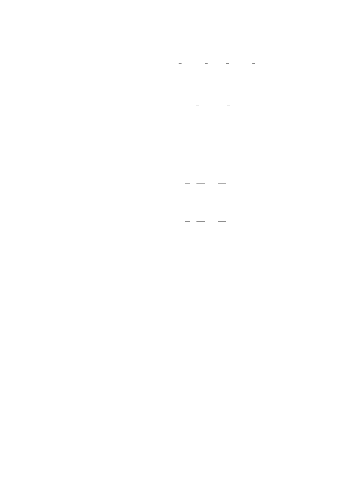
Then the total kinetic energy of the robotic arm is:
T = T
1
+ T
2
=
1
2
m
1
v
2
c1
+
1
2
I
1
.
q
2
1
+
1
2
m
2
v
2
c2
+
1
2
I
2
(
.
q
1
+
.
q
2
)
2
(2)
I
1
and I
2
represent the moments of inertia of the link about its center of mass. Since
both the upper arm and forearm rotate around their joints, the moments of inertia of the
upper arm and forearm are:
I
1
=
1
3
m
1
l
2
1
, I
2
=
1
3
m
2
l
2
2
(3)
The Lagrange function of the robotic arm is:
L = T − V =
1
2
(I
1
+ m
2
l
2
1
+ I
2
)
.
θ
2
1
+
1
2
I
2
.
θ
2
2
+ I
2
.
θ
1
.
θ
2
+ m
2
l
1
l
c2
.
θ
1
(
.
θ
1
+
.
θ
2
) cos θ
2
−
1
2
k(θ
2
− θ
o
)
2
(4)
Based on the Lagrange function, the Lagrange equations are further applied to each
generalized coordinate.
The Lagrange dynamic equation of the lower arm is:
d
dt
∂L
∂
.
q
1
!
−
∂L
∂q
1
= τ
1
(5)
The Lagrange dynamic equation of the upper arm is:
d
dt
∂L
∂
.
q
2
!
−
∂L
∂q
2
= τ
2
(6)
The dynamic model of the wafer transfer robot system is:
"
τ
1
τ
2
#
=
"
M
11
M
12
M
21
M
22
#"
..
q
1
..
q
2
#
+
"
C
11
C
12
C
12
C
22
#"
.
q
1
.
q
2
#
+
"
0
k(q
2
− θ)
#
(7)
In Equation (7), the stiffness term k(q
2
− θ
) represents the restoring torque induced
by the elastic deformation of the flexible transmission and is applied to the corresponding
joint equation.
3. Vibration Suppression Trajectory Planning for Robotic Arms Based on
Graylag Goose Algorithm
Existing robot trajectory planning methods include cubic and quintic polynomial
trajectory planning algorithms [
32
–
34
], T-shaped and S-shaped acceleration-deceleration
trajectory planning algorithms, and B-spline trajectory planning algorithms. During the
operation of a wafer handling manipulator, the start and end positions are known, while
the motion states during the process are unknown. This study uses a cubic polynomial
interpolation method to plan the motion trajectory [
35
]. This method combines the low
impact and high stability of S-shaped trajectory planning with the low computational
load of T-curve planning. It is easy to program and debug, has high reliability, and can
avoid sudden changes in acceleration, thereby effectively suppressing vibrations at the
manipulator’s end. As shown in Figure 2, the polynomial trapezoidal interpolation curve
trajectory is defined over the interval (0, t
6
). The robotic arm first experiences smooth
startup acceleration, the acceleration decreases beginning at time t
1
, and reaches constant
https://doi.org/10.3390/s26030829