s25061872.pdf - 第12页
Sensors 2025 , 25 , 1872 12 of 24 commonly used in machine learning, which is known as Bayesian optimization. The Gaussian process mainly includes Gaussian process r egression and an acquisition function. First, it estab…
Sensors 2025, 25, 1872
11 of 24
η
t
= η
min
+
1
2
(η
max
−η
min
) × (1 + cos(
T
cur
T
max
π)) (18)
where
η
t
is the current learning rate.
η
min
and
η
max
are the minimum and maximum values
of the learning rate, which are 0.001 and 0.01 in this paper. T
cur
and T
max
are the current
and total iterations, respectively. T
max
is usually set to half the number of iterations of the
main algorithm, which is 20 in this article [37].
Sensors2025,25,xFORPEERREVIEW 11 of 25
convergingonlocaloptima.Nonetheless,theimplementationofsuchspecializedlearn‐
ingmechanismsnotonlyentailsanotableincreaseinal gorithmiccomplexitybutalso
exhibitsdiminishedefficacywhenadaptingtothediversephasesoftheoptimizationpro‐
cedure.However,the SOalgorithmcan achieve aneffectivedynamicbalance
between
globalandlocalsearchesbydynamicallyadjustingthesefixedlearni ng factors C
1,C2,
andC
3,therebyimp rov in gtheperformanceandefficiencyofthealgorithm.Thecon‐
creteexpressionoftherandomdisturbanceisshowninEquations(16)and(17).InEqua‐
tion(19),alphaisusedtostoretheparametervaluesforlearningfactorsC
1,C2,andC3.
delta sigma randn
(16)
(1) ()alpha t alpha t delta
(17)
wheresigmarepresentstheamplitudeoftheperturbation.Itis0.1inthispaper[36].alpha
islimitedtoarangebetween0.01and1.Randomfunction‘randn’representsarandom
valuewithastandardnormaldistribution.
2.4.3.CosineAnnealingLearningRate
InEquations(12)–(15),thestrat egyforupdating
theindi vidualpositionsisrel‐
ativelysimple.Withoutconsideringadjustingthestrategyasaniterationprogress,theSO
algorithmmainlyreliesonthecurrentindividual’spositionandvelocityvectortodeter‐
minethenextindividual’sposition.Thismethodismorelikelytocausethealgorithmto
becomestuckina
locallyoptimalsolution.Toimprovetheupdatestrategyoftheoriginal
SOalgorithm,thisstudyintroducedacosinelearningannealingrate.Thisstrategysim‐
ulatesthedynamicadjustmentof thelearningratebasedonthecosinefunction,which
candynamicallyadjustthespeedofthepositionupdatingbasedonthenumber
ofitera‐
tions. In the early stages of the iteration, the learning rate can be reduced rapidly to
achievefastconvergence.Inthelaterstagesoftheiteration,fineadjustmentsaremadeto
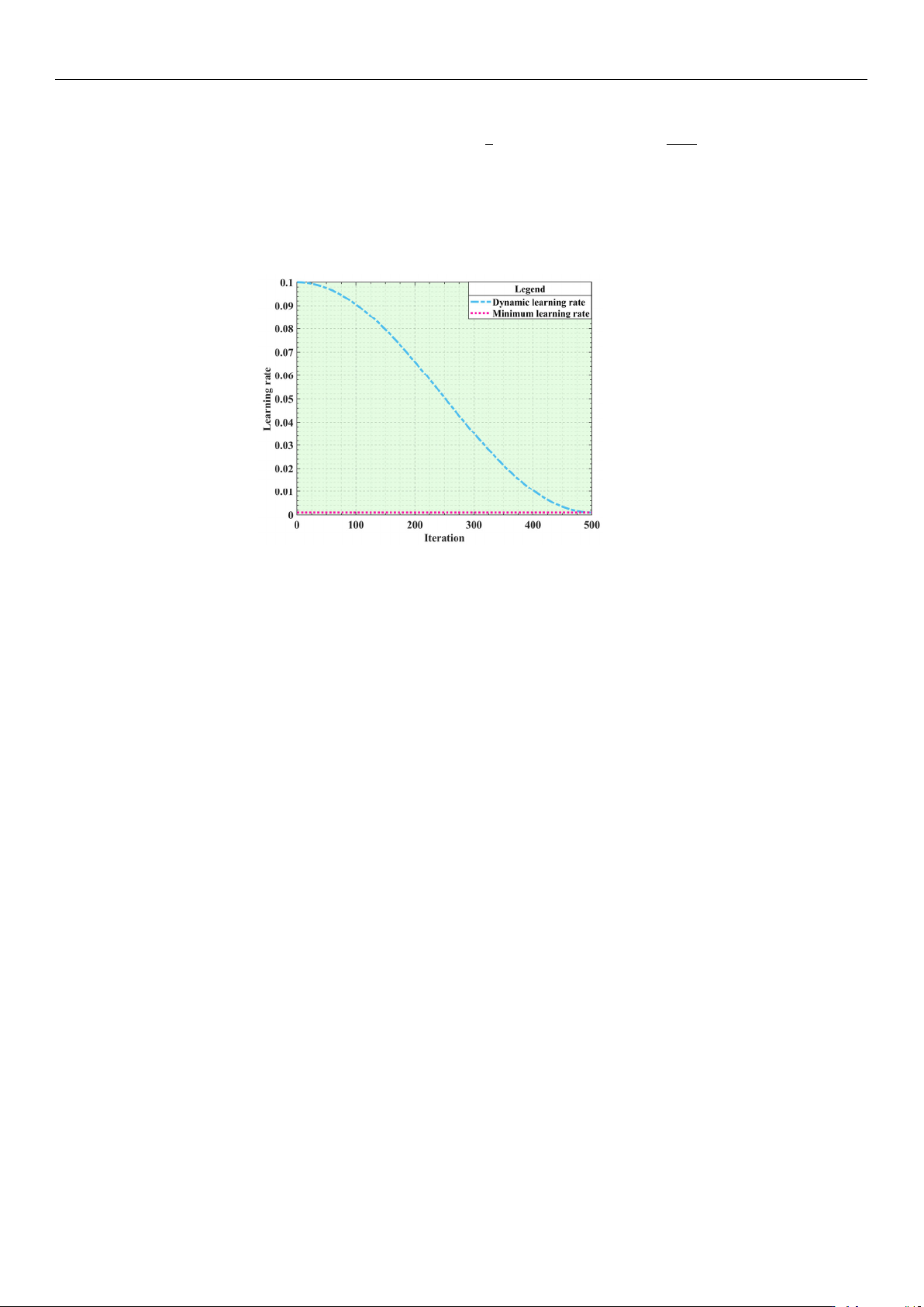
optimizetheprecisionofthesolutionbyreducingthelearningrate,asshowninFigure7.
The
specificexpressionofthecosinelearningannealingrateisshown inEqua tion(18).
min max min
max
1
()(1cos())
2
cur
t
T
T
(18)
whereη
tisthecurrentlearningrate.ηminandηmaxaretheminimumandmaximumvalues
ofthelearningrate,whichare0.001and0.01inthispaper.T
curandTmaxarethecurrent
andtotaliterations,respectively.T
maxisusuallysettohalfthenumberofiterationsofthe
mainalgorithm,whichis20inthisarticle[37].
Figure 7. Cosine annealing learning rate iteration graph.
By comparison with the cosine annealing learning rate, Gaussian adaptive param-
eters [
38
] are sensitive to initial conditions, prone to premature convergence, and may
introduce additional computational complexity. However, the cosine annealing learning
rate exhibits periodic change, which enables the SO algorithm to adopt diverse search strate-
gies in different stages, thus enhancing the dynamic adjustment ability of the algorithm.
This flexibility helps the algorithm to avoid premature convergence during the search pro-
cess, thereby increasing the possibility of finding a global optimal solution. Therefore, by
introducing the cosine annealing learning rate based on Equations (12)–(15), the improved
Equations (19)–(22) are obtained.
X
i, m_1
(t + 1) = η
t
× X
rand, m_1
(t) ± η
t
×C
2
× A
m
×
[
(ub − lb) ×rand + lb
]
(19)
X
i, m_2
(t + 1) = η
t
× X
food
(t) ± η
t
×C
3
×Temp ×rand ×
[
X
food
(t) − X
i, m
(t)
]
(20)
X
i, m_3
(t + 1) = η
t
× X
i, m_3
(t) ± η
t
×C
3
× F
m
×rand ×
h
Q × X
best, f
− X
i, m
(t)
i
(21)
X
i, m_3
(t + 1) = η
t
× X
i, m_3
(t) ± η
t
×C
3
× F
m
×rand ×
h
Q × X
best, f
− X
i, m
(t)
i
(22)
2.4.4. The Bayesian Method to Find the Optimization Threshold
Bayesian optimization can be applied not only to neural network architectures based
on snake algorithms to improve system performance [
39
], but also to optimize hyperpa-
rameter combinations in machine learning. In the process of determining threshold values
of the SO algorithm, parameter setting often depends on the experience and intuition
of algorithm developers or needs to be determined by practical users through practice.
This approach lacks universality and requires considerable time for experimentation and
adjustments. If the parameters are not selected properly, the adaptability of the algorithm
may be affected. To solve the problem in which the SO algorithm has difficulty adapting
parameters in the iterative process, this study introduces a hyperparameter-tuning method

Sensors 2025, 25, 1872
12 of 24
commonly used in machine learning, which is known as Bayesian optimization. The
Gaussian process mainly includes Gaussian process regression and an acquisition function.
First, it establishes prior knowledge of the global behavior of the objective function
through a Gaussian process. The mean vector and covariance matrix involved in the
prior distribution are shown in Equations (23) and (24). Subsequently, using the observed
objective function to obtain values at different input points, this prior knowledge is up-
dated to form a posterior distribution. The posterior mean and variance are given by
Equations (25) and (26).
Then, the improved collection function is expected to consider
the current best observations and the posterior distribution of the Gaussian process to
determine the next evaluation point. The collection function used in this study is expected
to improve equation shown in (27). In short, this method of guiding the search based on
existing knowledge can avoid many useless attempts.
µ
0
=
[
µ
0
(x
1
), . . . , µ
0
(x
k
)
]
T
(23)
∑
0
=
∑
0
(x
1
, x
1
) ···
∑
0
(x
1
, x
k
)
.
.
.
.
.
.
.
.
.
∑
0
(x
k
, x
1
) ···
∑
0
(x
k
, x
k
)
(24)
We assume that the above expression follows a multi-variate normal distribution,
where
µ
0
(x) represents the mean function.
∑
0
(x,x’) represents the kernel function, also
known as the covariance function, which describes the similarity between points x and x’
in the input space.
µ
n
(x) = µ
0
(x) +
∑
0
(x, x
1
: n) ×(K
x
1
:n,x
1
:n
+ σ
2
I)
−1
×( f (x
1
: n) −µ
0
(x
1
: n)) (25)
σ
2
n
(x) =
∑
0
(x, x) −
∑
0
(x, x
1
: n) ×(K
x
1
:n,x
1
:n
+ σ
2
I)
−1
×
∑
0
(x
1
, n : x) (26)
EI(x) = E
[
max
(
f (x) − f
∗
, 0
)]
(27)
where K
x
1:n,x1:n
is the kernel matrix.
σ
2
is the noise variance. f (x
1
:n) is the observed vector.
f * = max
i
= 1, . . . n is the currently observed best target value. f (x
i
) is the function value.
This study uses the ‘bayesopt’ function in MATLAB 2022B, which is an easy to use
and flexible Bayesian optimization tool. With the help of this tool, three key threshold
parameters (food threshold, temperature threshold and mating threshold) that affect the
balance between exploration and development in SO algorithm are mainly optimized. The
original parameter settings are 0.25, 0.6, and 0.6, respectively. Under an integrated Bayesian
optimization framework, they are redefined as three adjustable variables: threshold
1
,
threshold
2
, and threshold
3
. The construction of the parameter space is based on the original
thresholds, extending
±
0.2 on both sides, ensuring the validity of the parameters while
avoiding the computational burden caused by an overly large search space. Consider-
ing the characteristics of the low-dimensional parameter space, a Bayesian optimization
configuration with a maximum of 10 iterations is adopted in this study, which not only
guarantees optimization efficiency but also effectively saves computational resources.
The method establishes a cooperative mechanism between Bayesian optimization
framework based on Gaussian process and SO objective function, and realizes intelligent
optimization of optimal threshold combinations through parameter search strategy guided
by this model. To improve parameter generalization, K-fold cross-validation is employed
for robustness assessment. This approach partitions the dataset into K subsets, analyzing
performance variations across these subsets to effectively prevent overfitting and guide
optimization toward parameter configurations with enhanced generalization capabilities.
This safeguard mechanism not only enhances the reliability of parameter optimization
Sensors 2025, 25, 1872
13 of 24
but also provides theoretical support for the stable performance of the algorithm in un-
known scenarios.
2.4.5. ISO Algorithm Steps
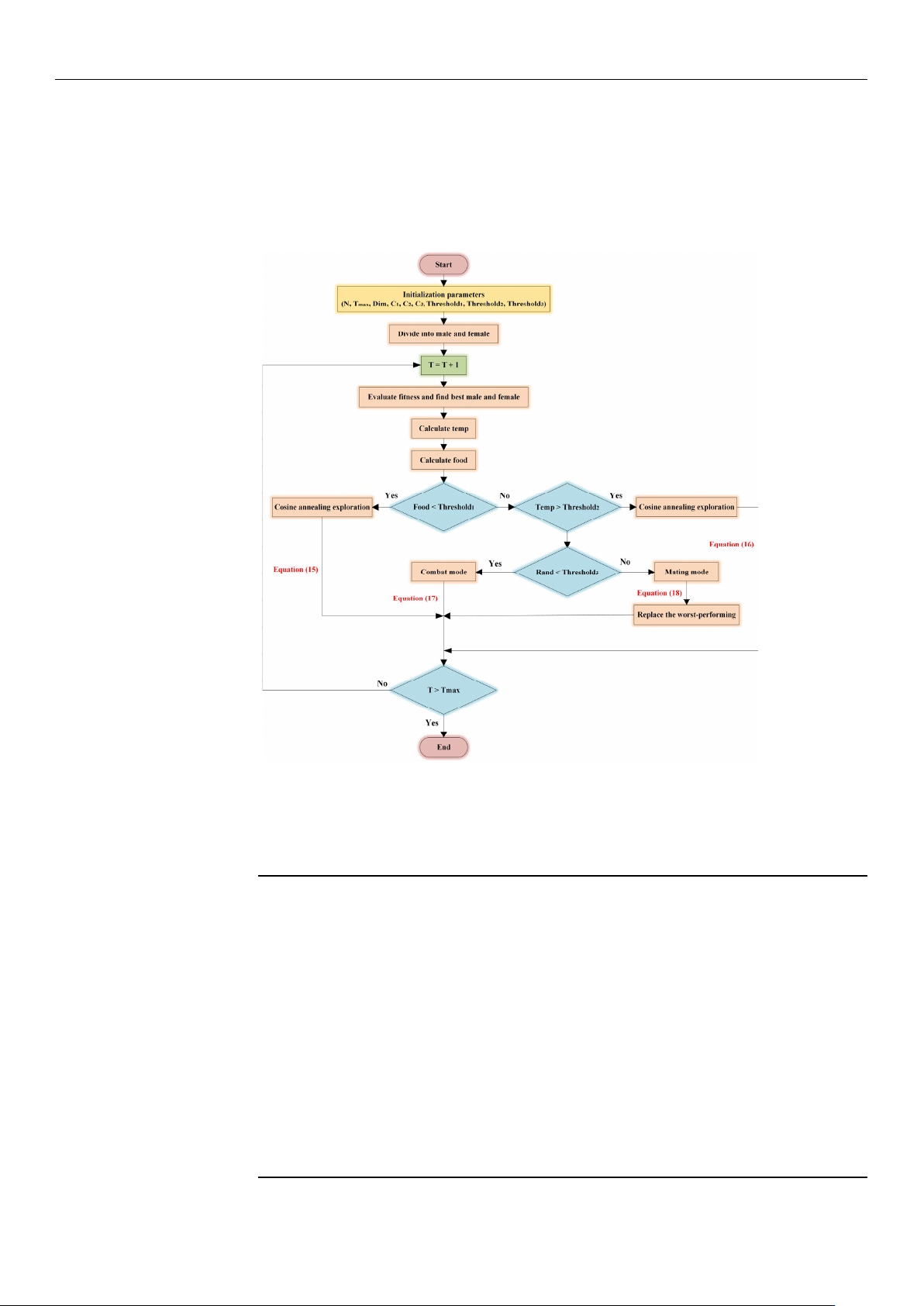
The flow chart of the ISO algorithm, which illustrates the step-by-step process, is
shown in Figure 8.
Sensors2025,25,xFORPEERREVIEW 14 of 25
Figure8.Theflowchartoftheimprovedsnakeoptimizationalgorithm.
TheISOalgorithmisoutlinedinAlgorithm,asshowninTable4.
Table4.ISOpseudo‐code.
1:Initializeparameters
2:InitializethepopulationusingtheTentChaoticMapasEquation(13)
3:DividepopulationintoN
mandNfusingEquations(10)and(11)
4:while(T<T
max)do
5:Evaluatethefitnessandidentifythebestfemaleandmale
6:CalculatetheiterationtemperatureandfoodquantityEquation(14)
7:if(Food<threshold
1)then
8:CosineannealingexplorationusingEquation(15)
9:elseif(Temp>threshold
2)then
10:CosineannealingexplorationusingEquation(16)
11:else
12:if(rand<threshold
3)then
13:EnterFightModeusingEquation(17)
14:else
15:EnterMatingModeusingEquation(18)
16:Replacetheworst‐performingfemaleandmale
Figure 8. The flow chart of the improved snake optimization algorithm.
The ISO algorithm is outlined in Algorithm, as shown in Table 4.
Table 4. ISO pseudo-code.
1: Initialize parameters
2: Initialize the population using the Tent Chaotic Map as Equation (13)
3: Divide population into N
m
and N
f
using Equations (10) and (11)
4: while (T < T
max
) do
5: Evaluate the fitness and identify the best female and male
6: Calculate the iteration temperature and food quantity Equation (14)
7: if (Food < threshold
1
) then
8: Cosine annealing exploration using Equation (15)
9: else if (Temp > threshold
2
) then
10: Cosine annealing exploration using Equation (16)
11: else
12: if (rand < threshold
3
) then
13: Enter Fight Mode using Equation (17)
14: else
15: Enter Mating Mode using Equation (18)
16: Replace the worst-performing female and male
17: end if
18: end if
19: end while
20: Return the optimal solution