s25061872.pdf - 第4页
Sensors 2025 , 25 , 1872 4 of 24 general, the points along the Z i axis are aligned with the i-th joint axis. Furthermore, the points along the X i axis are aligned with a common vertical line. In addition, the Y i axis …

Sensors 2025, 25, 1872
3 of 24
to overcome these shortcomings [
20
–
23
]. Lu and Wang [
24
] built an optimal trajectory
planning method based on a B-spline and a WOA to improve the work efficiency of a
robotic arm. However, they did not fully compare the performance differences between the
WOA and other existing algorithms. By combining the back propagation neural network
(BPNN) with the GA, the overall performance of the upper limb rehabilitation robotic arm
trajectory planning was improved to some extent. However, the parameter adjustment
after the combination was very complex and required a large number of experiments and
professional knowledge for correction [
25
]. The SO algorithm excels outstanding in the
realm of optimization owing to its exceptional flexibility and robustness. It is not only easy
to integrate chaos theory and learning mechanisms to bolster search efficiency but also
to maintain efficient exploration ability under poor initial conditions. In addition, it can
rapidly adapt to the changes in dynamic environments and optimize search strategies in
real time, thereby safeguarding the continuity and effectiveness of the optimization process.
Li et al. used a SO algorithm to find optimal paths in dynamic environments. Although its
performance has been improved compared with other intelligent algorithms, the improved
algorithm still requires careful parameter tuning [
26
]. To address the shortcomings of the
SO algorithm, recent literature [
27
,
28
] begun to focus on solving its core mechanism to
raise the overall performance of optimization problems. The ISO has also been gradually
applied to path planning and to solve general constrained optimization problems.
Therefore, considering the shortcomings of the afore-mentioned studies and the main
factors that should be prioritized during the actual operation of the wafer manipulator,
this study proposes an improved control strategy for a manipulator that combines the
single-segment start–stop S-shaped speed of the circular arc transition, an ISO algorithm,
and a time-impact optimization method of trajectory planning. It is worth noting that
it has more advantages in terms of the stability of the control effect or the convergence
ability of the algorithm compared with other types of methods. And it can adapt to
parameter optimization in different scenarios. In summary, the contributions of this study
are as follows.
(1)
In the area of intelligent optimization methods, the following improvements have
been made to the SO algorithm.
•
The Tent Chaotic Map initializes populations, instead of randomly generating
populations with ‘rand’ functions.
•
Dynamic learning factors, integrated with random perturbations, replace static
learning factors.
•
A cosine annealing learning rate scheme is employed for the adaptive updating
of individual positions.
•
The Bayesian method is utilized to optimize thresholds, surpassing the reliance
on empirical thresholds.
(2)
In the area of trajectory planning, the following improvements have been made to the
S-shaped speed curve.
• The interpolated arc transition supplants the abrupt right-angle transition.
•
The continuous single-segment start–stop mechanism supersedes the segmented
start–stop mechanism.
2. Materials and Methods
2.1. The Structure Parameters of the Wafer-Handling Robotic Arms
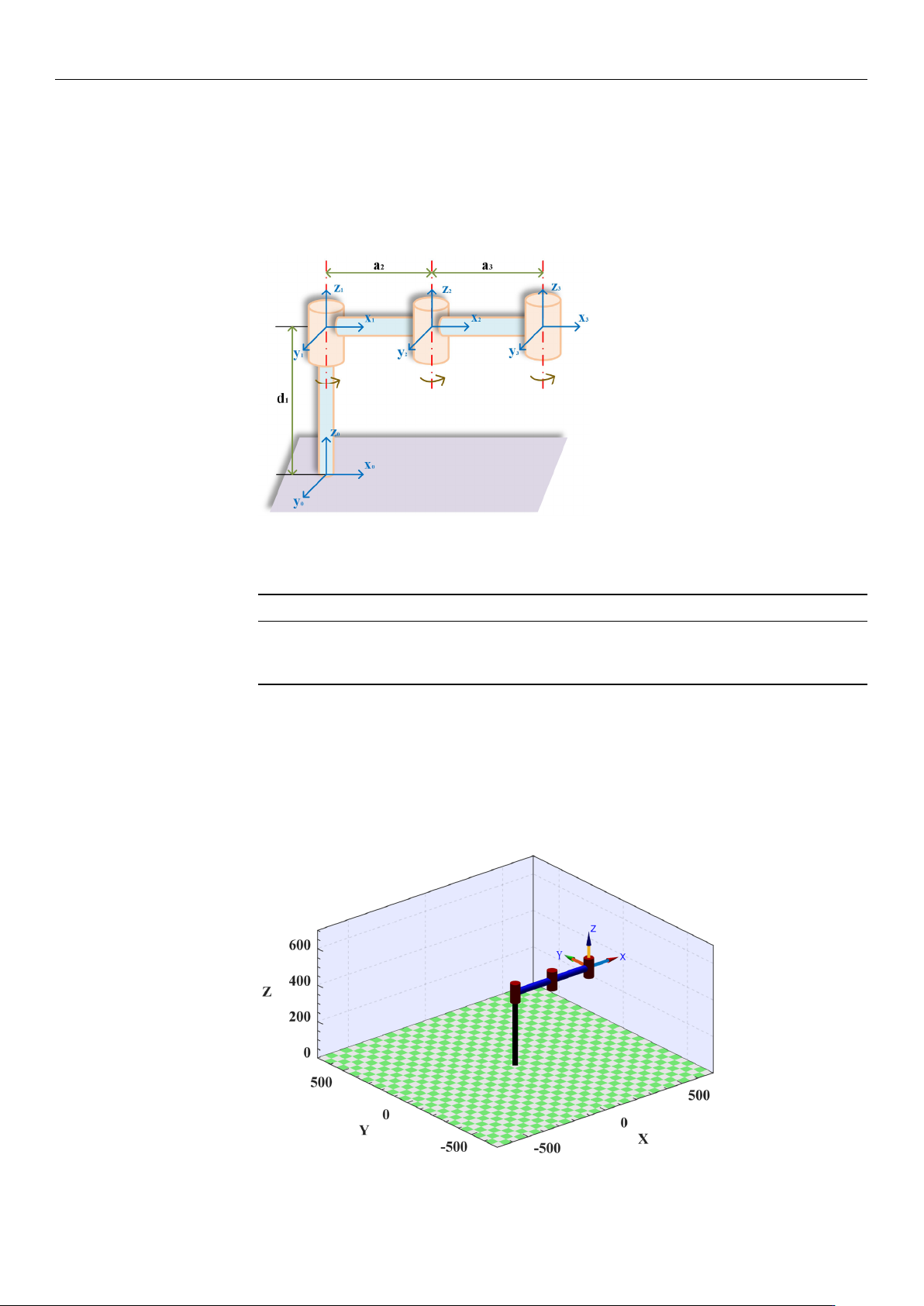
Assuming that the task requirements can be realized in a plane, the system model
is simplified when the robotic arm transports the wafer, as shown in Figure 1. Before
planning the trajectory, it is necessary to establish the link coordinate system correctly. In
Sensors 2025, 25, 1872
4 of 24
general, the points along the Z
i
axis are aligned with the i-th joint axis. Furthermore, the
points along the X
i
axis are aligned with a common vertical line. In addition, the Y
i
axis is
oriented according to the right-hand rule. In this study, the parameters of the linkage rods
are expressed using the improved Denavit–Hartenberg (DH) method. The parameters of
each joint and link are obtained using the link coordinate system as a reference, as shown
in Table 1.
Sensors2025,25,xFORPEERREVIEW 4 of 25
2.MaterialsandMethods
2.1.TheStructureParametersoftheWafer‐HandlingRoboticArms
Assumingthatthetaskrequirementscanberealizedinaplane,thesystemmodel
issimplifiedwhentheroboticarmtransportsthewafer,asshowninFigure1.Beforeplan‐
ningthetrajectory,itisnecessarytoestablishthelink
coordinatesystemcorrectly.Ingen‐
eral,thepointsalongtheZ
iaxisarealignedwiththei‐thjointaxis.Furthermore,thepoints
alongtheX
i axisarealignedwitha comm on vert ical line. In addition, the Yiaxisis
orientedaccordingtotheright‐handrule.Inthisstudy,theparametersofthelinkagerods
areexpressedusingtheimprovedDe navit–Hartenberg(DH) method.Theparameters
of each joint and linkare obtained using the link coordinatesystem as a reference, as
showninTable1.
Figure1.Simplifiedmodelofthewafer‐handlingroboticarm.
Table1.Linkageparametersofthe3Rroboticarm.
Linki ai/mmαi/(°) di/mmθi(/°) Rangeofθi/(°)
1 0 0 400 0 −120–120
2 0 238.4 0 0 −120–120
3 0 238.4 0 0 −120–120
Tofacilitatethevisualanalysisofthesubsequenttrajectoryplanningandverifythe
correctnessofthesimplifiedmodel,thisstudyutilizestheMATLABrobottoolboxdevel‐
opedbyPeterCorke.Itisapowerfulroboticsimulationandanalysistoolthatprovidesa
rangeofcapabilitiesformodeling,simulating,controlling,and
visualizingrobots.Aro‐
boticarmconsistentwiththesimplifiedmodelissuccessfullyconstructedontheinterface
byfollowingthebuildinginstructionsintheMATLABrobottoolbox,asshowninFigure
2.
Figure 1. Simplified model of the wafer-handling robotic arm.
Table 1. Linkage parameters of the 3R robotic arm.
Link
i
a
i
/mm α
i
/(
◦
) d
i
/mm θ
i
(/
◦
) Range of θ
i
/(
◦
)
1 0 0 400 0 −120–120
2 0 238.4 0 0 −120–120
3 0 238.4 0 0 −120–120
To facilitate the visual analysis of the subsequent trajectory planning and verify the
correctness of the simplified model, this study utilizes the MATLAB robot toolbox devel-
oped by Peter Corke. It is a powerful robotic simulation and analysis tool that provides a
range of capabilities for modeling, simulating, controlling, and visualizing robots. A robotic
arm consistent with the simplified model is successfully constructed on the interface by
following the building instructions in the MATLAB robot toolbox, as shown in Figure 2.
Sensors2025,25,xFORPEERREVIEW 5 of 25
Figure2.Wafer−handlingroboticarminMATLAB.
2.2.TheMathematicalModelofMultipleObjectiveFunction
Inrecentyears,theoptimizationoftime,energy,impact,andotherindicatorshas
beenshowntoimprovetheoperationalefficiencyandmotionperformanceofroboticarms
inthefieldofrobottrajectoryplanning[29–31].Inthepreprocessingstageoftrajectory
optimization
analysis,expected traject ori es asinputpara meters needtobepr edefined
and generated. Therefore, this study will build the expected trajectory through the
MATLABplatform,andthespecificimplementationprocesswillbeelaboratedinthefol‐
lowing sections. Considering the production background and opt imization effect, a
multi‐segmentpoint‐to
‐poi nt trajectoryinCartesianspaceisadoptedtoachievemulti‐
objectiveoptimizationoftimeandimpact.Inthefollowingsection,wewillsystematically
analyzethemathematicalmodelanditsoptimizationprocess.
Initially,thedesiredtrajectoryoftheroboticarmisdiscretizedintomultipleinterpo‐
lationpointswithintheCartesianspace.
Theseinterpolationpointsareselectedatregular
timeintervalsalongthedesired trajectory,therebya ccurate lycapturingtheposit i ona l
informationofthetrajectoryatdifferenttimeinstances.Subsequently,theCartesiancoor‐
dinatesoftheseinterpolationpointsarestoredinthejointcontroller.Byemployingthe
inversekinematicsequations,theCartesiancoordinates
oftheinterpolationpointscanbe
furthertransformedintothecorrespondingjointanglesinthejointspace.However,the
inversekinematicsequationstypicallyyieldtwodistinctsolutions.Therefore,itisneces‐
sarytoimposegeometricconstraintswithinthecodetoselecttheuniquesolutionthat
conformstothedesiredtrajectory.
Oncetheuniquesolutionisobtained,itissubstituted
intothe robot’s forward kinemati cs model to deri ve theCartesian coordinatesofthe
desiredtraject ory.Ulti mately,bycombin i ngthe trajectory fu nctionwiththeCartesian
coordinatesoftheinterpolationpoints,thedesiredtrajectoryispreciselyreconstructed.It
isassumedthatthetimeat
whichthemanipulatorreacheseachinterpolationpointist
i
.
Thetimeintervalbetweenadjacentinterpolationpoints ish
i
=t
i+1
−t
i
,whereiistheindex
oftheinterpolationpo ints(i=0,1,…n).Theti meint ervaltakeninthecodeofthispaper
is0.002s,thatis,theselectionbasis ofinterpolationpoints.Atthesa metime,through
thepreliminaryanalysis,itisclearlyobservedthat
thereisaninversecorrelationbetween
timeandimpact.Whenthetimeoftheroboticarmincreases,theimpactdecreases.
Therefore,itisimpossibletosimultaneouslyobtaintheminimu mvalues.Thus, con‐
sideringtheconstraintsofthegeometricjointsoftheroboticarm,velocity,accelera‐
tion,andjerk,theprimarygoal
ofthisstudyistoachieveanoptimalbalancebetweentime
andimpact.Therefore,a Paretooptimalmethodisadoptedinthisstudytoachieve the
tradeoffbetweenoptimizationobjectives.ThetimefunctionisgivenbyEquation(1).
Figure 2. Wafer−handling robotic arm in MATLAB.

Sensors 2025, 25, 1872
5 of 24
2.2. The Mathematical Model of Multiple Objective Function
In recent years, the optimization of time, energy, impact, and other indicators has been
shown to improve the operational efficiency and motion performance of robotic arms in the
field of robot trajectory planning [
29
–
31
]. In the preprocessing stage of trajectory optimiza-
tion analysis, expected trajectories as input parameters need to be predefined and generated.
Therefore, this study will build the expected trajectory through the MATLAB platform, and
the specific implementation process will be elaborated in the following sections. Consider-
ing the production background and optimization effect, a multi-segment point-to-point
trajectory in Cartesian space is adopted to achieve multi-objective optimization of time and
impact. In the following section, we will systematically analyze the mathematical model
and its optimization process.
Initially, the desired trajectory of the robotic arm is discretized into multiple interpola-
tion points within the Cartesian space. These interpolation points are selected at regular
time intervals along the desired trajectory, thereby accurately capturing the positional infor-
mation of the trajectory at different time instances. Subsequently, the Cartesian coordinates
of these interpolation points are stored in the joint controller. By employing the inverse
kinematics equations, the Cartesian coordinates of the interpolation points can be further
transformed into the corresponding joint angles in the joint space. However, the inverse
kinematics equations typically yield two distinct solutions. Therefore, it is necessary to
impose geometric constraints within the code to select the unique solution that conforms to
the desired trajectory. Once the unique solution is obtained, it is substituted into the robot’s
forward kinematics model to derive the Cartesian coordinates of the desired trajectory.
Ultimately, by combining the trajectory function with the Cartesian coordinates of the
interpolation points, the desired trajectory is precisely reconstructed. It is assumed that
the time at which the manipulator reaches each interpolation point is t
i
. The time interval
between adjacent interpolation points is h
i
= t
i+
1
−
t
i
, where i is the index of the interpola-
tion points (i = 0, 1, . . . n). The time interval taken in the code of this paper is 0.002 s, that
is, the selection basis of interpolation points. At the same time, through the preliminary
analysis, it is clearly observed that there is an inverse correlation between time and impact.
When the time of the robotic arm increases, the impact decreases. Therefore, it is impossible
to simultaneously obtain the minimum values. Thus, considering the constraints of the
geometric joints of the robotic arm, velocity, acceleration, and jerk, the primary goal of
this study is to achieve an optimal balance between time and impact. Therefore, a Pareto
optimal method is adopted in this study to achieve the tradeoff between optimization
objectives. The time function is given by Equation (1). Because the impact quantity can
not be directly measured, it is quantified by the acceleration, as shown in Equation (2).
The constraints are expressed in Equation (3). The multi-objective optimization function is
shown in Equation (4).
minF
1
=
n
∑
i=0
h
i
(1)
minF
2
=
n
∑
i=0
s
R
t
i
0
j
2
i
dt
t
i
(2)
|
θ
i
|
≤ θ
max
|
v
i
|
≤ v
max
|
a
i
|
≤ a
max
|
j
i
|
≤ j
max
(3)
minF = w
1
·
|
F
1
− F
1min
|
+ w
2
·
|
F
2
− F
2min
|
(4)