s25061872.pdf - 第6页
Sensors 2025 , 25 , 1872 6 of 24 where F 1 , F 1 min , and w 1 are the objective function, minimum value, and weight value of time, respectively . F 2 , F 2 min , and w 2 are the objective function, minimum value, and we…

Sensors 2025, 25, 1872
5 of 24
2.2. The Mathematical Model of Multiple Objective Function
In recent years, the optimization of time, energy, impact, and other indicators has been
shown to improve the operational efficiency and motion performance of robotic arms in the
field of robot trajectory planning [
29
–
31
]. In the preprocessing stage of trajectory optimiza-
tion analysis, expected trajectories as input parameters need to be predefined and generated.
Therefore, this study will build the expected trajectory through the MATLAB platform, and
the specific implementation process will be elaborated in the following sections. Consider-
ing the production background and optimization effect, a multi-segment point-to-point
trajectory in Cartesian space is adopted to achieve multi-objective optimization of time and
impact. In the following section, we will systematically analyze the mathematical model
and its optimization process.
Initially, the desired trajectory of the robotic arm is discretized into multiple interpola-
tion points within the Cartesian space. These interpolation points are selected at regular
time intervals along the desired trajectory, thereby accurately capturing the positional infor-
mation of the trajectory at different time instances. Subsequently, the Cartesian coordinates
of these interpolation points are stored in the joint controller. By employing the inverse
kinematics equations, the Cartesian coordinates of the interpolation points can be further
transformed into the corresponding joint angles in the joint space. However, the inverse
kinematics equations typically yield two distinct solutions. Therefore, it is necessary to
impose geometric constraints within the code to select the unique solution that conforms to
the desired trajectory. Once the unique solution is obtained, it is substituted into the robot’s
forward kinematics model to derive the Cartesian coordinates of the desired trajectory.
Ultimately, by combining the trajectory function with the Cartesian coordinates of the
interpolation points, the desired trajectory is precisely reconstructed. It is assumed that
the time at which the manipulator reaches each interpolation point is t
i
. The time interval
between adjacent interpolation points is h
i
= t
i+
1
−
t
i
, where i is the index of the interpola-
tion points (i = 0, 1, . . . n). The time interval taken in the code of this paper is 0.002 s, that
is, the selection basis of interpolation points. At the same time, through the preliminary
analysis, it is clearly observed that there is an inverse correlation between time and impact.
When the time of the robotic arm increases, the impact decreases. Therefore, it is impossible
to simultaneously obtain the minimum values. Thus, considering the constraints of the
geometric joints of the robotic arm, velocity, acceleration, and jerk, the primary goal of
this study is to achieve an optimal balance between time and impact. Therefore, a Pareto
optimal method is adopted in this study to achieve the tradeoff between optimization
objectives. The time function is given by Equation (1). Because the impact quantity can
not be directly measured, it is quantified by the acceleration, as shown in Equation (2).
The constraints are expressed in Equation (3). The multi-objective optimization function is
shown in Equation (4).
minF
1
=
n
∑
i=0
h
i
(1)
minF
2
=
n
∑
i=0
s
R
t
i
0
j
2
i
dt
t
i
(2)
|
θ
i
|
≤ θ
max
|
v
i
|
≤ v
max
|
a
i
|
≤ a
max
|
j
i
|
≤ j
max
(3)
minF = w
1
·
|
F
1
− F
1min
|
+ w
2
·
|
F
2
− F
2min
|
(4)
Sensors 2025, 25, 1872
6 of 24
where F
1
, F
1min
, and w
1
are the objective function, minimum value, and weight value of
time, respectively. F
2
, F
2min
, and w
2
are the objective function, minimum value, and weight
of impact, respectively. h
i
is the time interval between the i-th and i + 1-th interpolation
point. t
i
and j
i
denote the time node and jerk value of the i-th interpolation point.
θ
max
,
v
max
, a
max
, and j
max
are the maximum rotational angle, speed, acceleration, and jerk of the
joint of the manipulator arm, respectively.
2.3. The Construction of Trajectory Planning
2.3.1. The Explanation of S-Shaped Speed Curve
The T-shaped speed curve is a widely used method for robotic arm control. Because
of its simplicity and ease of control, it is extremely common in industrial applications.
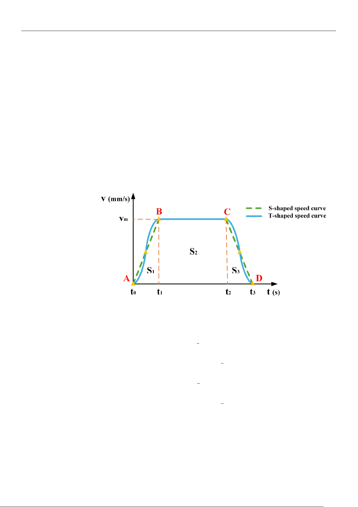
As shown in Figure 3, this curve may produce large impacts and vibrations at points
A, B, C, and D, potentially causing the wafer to break. By contrast, the S-shaped speed
curve uses nonlinear adjustments to increase and decrease the velocity, making the motion
process smoother and effectively solving the discontinuity problem of the acceleration of
the
T-shaped
speed curve. Therefore, the S-shaped speed curve is more suitable in scenarios
requiring higher operational stability.
Sensors2025,25,xFORPEERREVIEW 7 of 25
localtimeperiodofpartk,whichreferstothedifferencefromthestartingpointofthe
currentpart,calledtimezero,tothetimepointofthecurrentpart.Theequationused
τ
k = tk−tk−1(k=1,2,…7). vk ( k=1,2,…6)representsthefinalspeed ofpart kandvs.
repres entsthei nitialspeed.a
maxisthemaximumacceleration.jmaxisthemaximumaccel‐
eration.
Figure3.CorrelationchartbetweentheT‐shapedandS‐shapedspeedcurves.
2.3.2.TheImprovementoftheS‐ShapedSpeedCurve
Trajectoryplanningisacrucialstepintheroboticmotioncontrol.Whenthewafer‐
handlingroboticarmisinoperation,itfrequentlyencountersturningpointswherethe
directionofmovementrequiresalteration.Theseturningpointsoftenserveasasourceof
abrupt
jerkchanges.Toalleviatethisproblem,anS‐shapedspeedcurveadopts acircular
arctransitionstrategytoguaranteeasmoothtrajectorytransition.Thisstrategynotonly
mitigates the impact and vibrationinduced by therobotic arm but also contributes to
shorteningtheexecutiontimeofthemotiontrajectory.Prior
toconstructingtheS‐shaped
speedcurve,itisimperativetodeterminethekeyinterpolationpointsofthetrajectoryin
Cartesianspace,asindicatedinTable2.Simultaneously,theprincipal motionparameters
mustbesetaspresentedinTable3.v_p
0,v_p1,andv_p2arethevelocitiesoftheinitial
point,thecirculararctransitionsection,andtheterminalpoint,respectively.v
max,amax,and
jmaxdenotethemaximumvelocity,themaximumacceleration,andthemaximumrateof
changeintheaccelerationofanendeffectorinCartesianspace,respectively.ristheradius
ofthecirculararctransitionattheinflectionpoint.
Table2.SegmentationpointsinCartesianspace.
StartingPoint IntermediatePoint EndingPoint
(400,0,400) (200,0,400) (200,200,400)
Table3.ThemainmotionparametersoftheS‐shapedspeedcurve.
v_p0
(mm/s)
v_p
1
(mm/s)
v_p
2
(mm/s)
v
max
(mm/s)
a
max
(mm/s
2
)
j
max
(mm/s
3
)
r
(mm)
0 100 0 100 100 100 30
ThetrajectorycurveshowninFigure4.canbegeneratedby applyingtheparameters
listedin Table 3. to the S‐shaped speedcurve model. In thisfigure, the black lines
represent the direct path without a circular transition, whereas the blue lines show a
smoothpathwitha circulartra nsiti on.
Itisno te wort hythattheradiusofthecircular
Figure 3. Correlation chart between the T-shaped and S-shaped speed curves.
The S-shaped speed curve partitions the entire motion process into seven distinct
phases. Equation (5) describes the motion characteristics at different stages.
v(t) =
v
s
+
1
2
j
max
τ
2
1
0 ≤ t ≤ t
1
v
1
+ a
max
τ
2
t
1
≤ t ≤ t
2
v
2
+ a
max
τ
3
−
1
2
j
max
τ
2
3
t
2
≤ t ≤ t
3
v
3
t
3
≤ t ≤ t
4
v
4
−
1
2
j
max
τ
2
5
t
4
≤ t ≤ t
5
v
5
− a
max
τ
6
t
5
≤ t ≤ t
6
v
6
− a
max
τ
7
+
1
2
j
max
τ
2
7
t
6
≤ t ≤ t
7
(5)
where t
k
(k = 0, 1, . . . 7) represents the transition point time of part k, which indicates the specific
point in time at which each stage begins or ends.
τ
k
(k = 0, 1, .. . 7) represents the local time
period of part k, which refers to the difference from the starting point of the current part, called
time zero, to the time point of the current part. The equation used
τ
k
= t
k
− t
k−
1
(k = 1, 2, .. . 7).
v
k
(k = 1, 2, . . . 6) represents the final speed of part k and vs. represents the initial speed. a
max
is
the maximum acceleration. j
max
is the maximum acceleration.

Sensors 2025, 25, 1872
7 of 24
2.3.2. The Improvement of the S-Shaped Speed Curve
Trajectory planning is a crucial step in the robotic motion control. When the wafer-
handling robotic arm is in operation, it frequently encounters turning points where the
direction of movement requires alteration. These turning points often serve as a source of
abrupt jerk changes. To alleviate this problem, an S-shaped speed curve adopts a circular
arc transition strategy to guarantee a smooth trajectory transition. This strategy not only
mitigates the impact and vibration induced by the robotic arm but also contributes to
shortening the execution time of the motion trajectory. Prior to constructing the S-shaped
speed curve, it is imperative to determine the key interpolation points of the trajectory in
Cartesian space, as indicated in Table 2. Simultaneously, the principal motion parameters
must be set as presented in Table 3. v_ p
0
, v_ p
1
, and v_ p
2
are the velocities of the initial
point, the circular arc transition section, and the terminal point, respectively. v
max
, a
max
, and
j
max
denote the maximum velocity, the maximum acceleration, and the maximum rate of
change in the acceleration of an end effector in Cartesian space, respectively. r is the radius
of the circular arc transition at the inflection point.
Table 2. Segmentation points in Cartesian space.
Starting Point Intermediate Point Ending Point
(400, 0, 400) (200, 0, 400) (200, 200, 400)
Table 3. The main motion parameters of the S-shaped speed curve.
v_ p
0
(mm/s)
v_ p
1
(mm/s)
v_ p
2
(mm/s)
v
max
(mm/s)
a
max
(mm/s
2
)
j
max
(mm/s
3
)
r
(mm)
0 100 0 100 100 100 30
The trajectory curve shown in Figure 4. can be generated by applying the parameters
listed in Table 3. to the S-shaped speed curve model. In this figure, the black lines represent
the direct path without a circular transition, whereas the blue lines show a smooth path
with a circular transition. It is noteworthy that the radius of the circular transition can be
adjusted according to specific work requirements. Overall, the circular transition not only
improves the smoothness and efficiency of the robotic arm’s motion but also helps to protect
the robotic arm and its payload, while enhancing the overall operational performance.
This transition method allows the robotic arm to perform complex tasks more accurately
and reliably.
Sensors2025,25,xFORPEERREVIEW 8 of 25
transitioncanbeadjustedaccordingtospecificworkrequirements.Overall,thecircular
transitionnotonlyimprovesthesmoothnessandefficiencyoftheroboti carm’smotion
but also helpstoprotectthe roboticarmandits payload, whileenhancing the overall
operational performance. This transition method allows the robotic arm
to pe rf or m
complextasksmoreaccuratelyandreliably.
Figure4.Contrastdiagramofarctransitionandright‐anglepath.
ByanalyzingthedatainTable2,itisclearthatthistrajectoryplanningtaskinvolves
threekeynodesthattheroboticarmmustreachinsequence.S‐shapedspeedcurve
planningisastandardpoint‐to‐pointstart–stopmotionscheme.Specifically,thistaskis
representedbytwomovementsfrom
thestartingpointtothemiddlepoint andthen
fromthemiddlepointtotheendpoint,withzerostartingandendingspeedsforeach
movement.BasedonthedatainTable3,thevelocityimageoftheschemeisshownin
Figure5.However,thisschemecausesthemanipulator
tofrequentlystartandstop,which
notonlyincreasesthevibrationduringthemotionprocessbutalsoleadstotimewastage
intheaccelerationanddecelerationstages.Toaddressthisissue,animprovedschemeis
proposed in this study for the single‐segment start–st op mechanism, optimizing the
startingandstoppingparts
oftheintermediateprocessintoasmoothmotionmodewith
constantspeedsatbothends,asshowninFigure6.Whenthevelocityofthefirstsegment
ofmotionattainsthemaximumva lueofthesetparameters,insteadof reducingthe
velocitybacktozeroasinthestandardscheme,
thesecondsegmentofmotionproceeds
inauniformtransitionmanner.Thespecificpara mete rsstillrefertoTable 3.This
improved scheme effectively mitigates the limitations inherent in the conventiona l
approach.Simultaneously,themovementefficiencycanbeimprovedand thevi bra ‐
tioncanbereduced.
Figure5.Thecontinuousstart–stopS‐shapedspeedcurve.
Figure 4. Contrast diagram of arc transition and right-angle path.