s25061872.pdf - 第16页
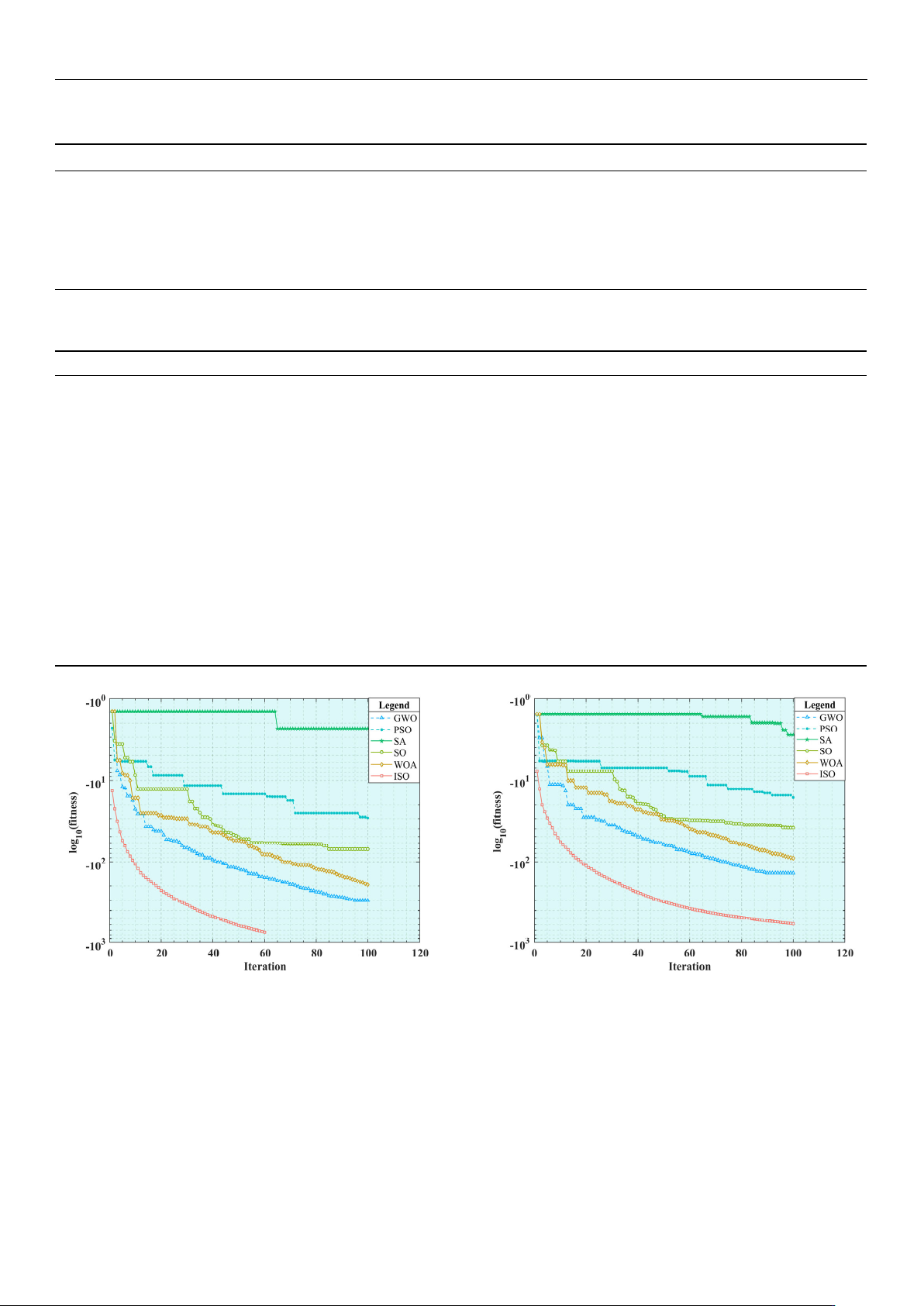
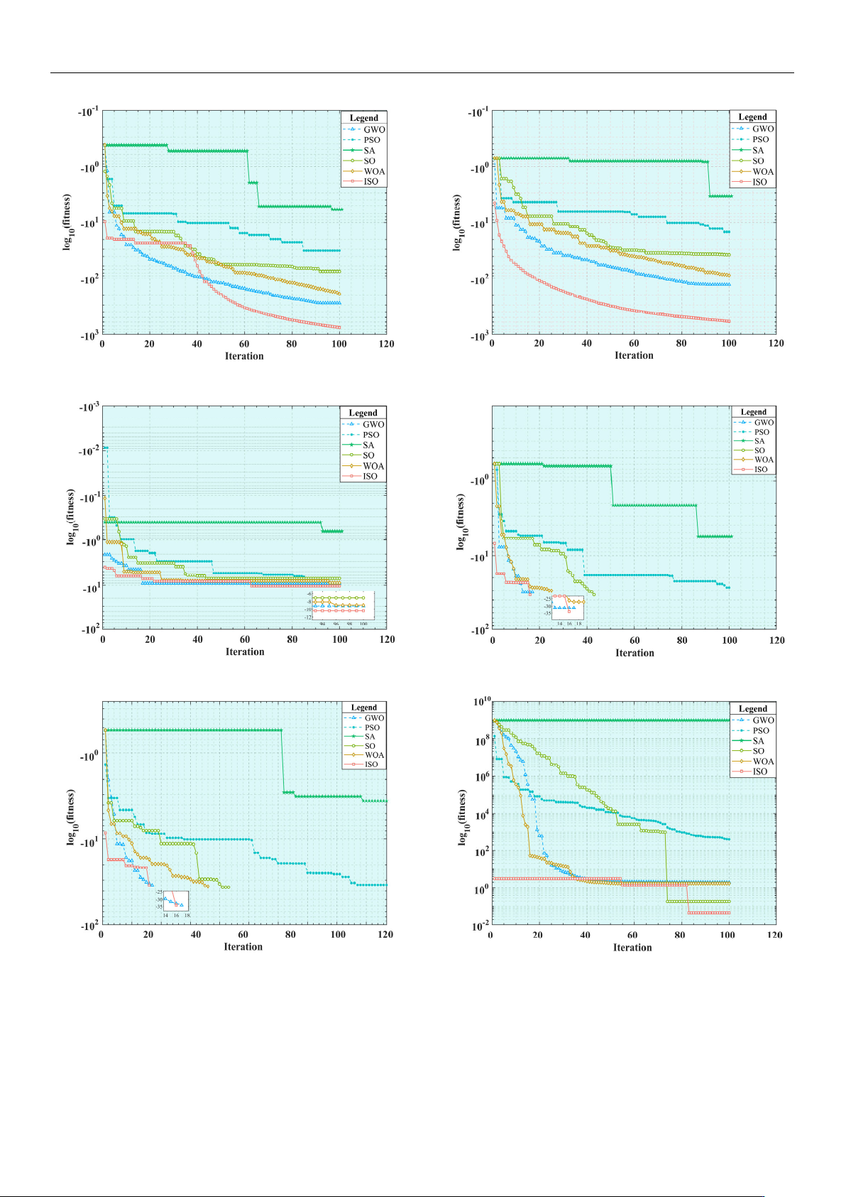
Sensors 2025 , 25 , 1872 16 of 24 Sensors 2025 , 25 , x FOR PE ER REV I E W 17 of 25 ( c ) ( d ) ( e ) ( f ) ( g ) ( h ) Figure 9. Convergence cu rve of the ref…
Sensors 2025, 25, 1872
15 of 24
Table 6. Parameter settings for the algorithms.
Algorithm Parameter Settings
SO Theshold
1
= 0.25, Theshold
2
= 0.6, Theshold
3
= 0.6, C
1
= 0.5, C
2
= 0.05, C
3
= 2
SA Temp = 100, Temp
min
= 0.01, alpha = 0.95
PSO w = 0.9, c
1
= 2, c
2
= 2, V
max
= 0.3 ∗ ub, V
min
= 0.3 ∗ lb
GWO r
1
= r
2
= rand
WOA r
1
= r
2
= rand, p = rand, b = 1
ISO sigma = 0.1, alpha
min
= 0.01, alpha
max
= 1.0, eta
max
= 0.01, eta
min
= 0.001
Table 7. Results obtained by different algorithms (D = 30).
Function SO SA PSO GWO WOA ISO
F
1
MEAN
8.27 × 10
−40
7.30 × 10
−2
3.04 × 10
−12
6.24 × 10
−105
8.40 × 10
−79
0
STD
2.51 × 10
−39
2.27 × 10
−1
6.51 × 10
−12
2.79 × 10
−104
2.10 × 10
−78
0
F
2
MEAN
3.95 × 10
−21
4.26 × 10
−2
1.38 × 10
−7
8.55 × 10
−57
2.95 × 10
−40
9.14 × 10
−214
STD
5.26 × 10
−21
2.87 × 10
−2
2.22 × 10
−7
3.13 × 10
−56
7.95 × 10
−40
0
F
3
MEAN
2.16 × 10
−39
3.85 × 10
−2
6.47 × 10
−12
6.66 × 10
−107
2.18 × 10
−79
0
STD
7.04 × 10
−39
8.37 × 10
−2
2.16 × 10
−11
2.98 × 10
−106
6.74 × 10
−79
0
F
4
MEAN
2.01 × 10
−20
1.34 × 10
−1
1.38 × 10
−6
1.27 × 10
−53
8.56 × 10
−40
2.27 × 10
−213
STD
3.54 × 10
−20
9.71 × 10
−2
2.36 × 10
−6
3.93 × 10
−53
2.64 × 10
−39
0
F
5
MEAN
7.01 × 10
−4
6.64 × 10
−1
1.77 × 10
−3
5.21 × 10
−4
7.33 × 10
−4
1.75 × 10
−4
STD
7.23 × 10
−4
8.91 × 10
−1
1.26 × 10
−3
5.08 × 10
−4
7.05 × 10
−4
2.72 × 10
−4
F
6
MEAN 0
1.79 × 10
−2
2.39 × 10
−12
0 0 0
STD 0
3.42 × 10
−2
3.35 × 10
−12
0 0 0
F
7
MEAN 0
1.67 × 10
−2
6.15 × 10
−12
0 0 0
STD 0
3.42 × 10
−2
3.35 × 10
−12
0 0 0
F
8
MEAN
1.74 × 10
1
1.10 × 10
9
4.41 × 10
1
1.24 × 10
0
8.13 × 10
−1
2.06 × 10
−1
STD
3.32 × 10
1
1.35 × 10
8
2.59 × 10
1
4.26 × 10
−1
3.08 × 10
−1
2.03 × 10
−1
Sensors2025,25,xFORPEERREVIEW 16 of 25
222 22
81
1
1
( ) 0.1 sin (3 ) ( 1) 1 sin (3 1) ( 1) 1 sin ( 2 )
( ,5,100, 4),
(),
(,,,) 0,
(),
n
iin n
i
n
i
i
m
ii
ii
m
ii
Fx x x x x x
ux
kx a x a
ux akm a x a
kxa x a
[−50,50] 0
Table6.Parameterseingsforthealgorithms.
Algorithm ParameterSeings
SO Theshold1=0.25,Theshold2=0.6,Theshold3=0.6,C1=0.5,C2=0.05,C3=2
SA Temp=100,Tempmin=0.01,alpha=0.95
PSO w=0.9,c
1=2,c2=2,Vmax=0.3*ub,Vmin=0.3*lb
GWO r
1=r2=rand
WOA r
1=r2=rand,p=rand,b=1
ISO sigma=0.1,alpha
min=0.01,alphamax=1.0,etamax=0.01,etamin=0.001
Table7.Resultsobtainedbydifferentalgorithms(D=30).
Function SO SA PSO GWO WOA ISO
F1
MEAN 8.27×10
−40
7.30×10
−2
3.04×10
−12
6.24×10
−105
8.40×10
−79
0
STD 2.51×10
−39
2.27×10
−1
6.51×10
−12
2.79×10
−104
2.10×10
−78
0
F
2
MEAN 3.95×10
−21
4.26×10
−2
1.38×10
−7
8.55×10
−57
2.95×10
−40
9.14×10
−214
STD 5.26×10
−21
2.87×10
−2
2.22×10
−7
3.13×10
−56
7.95×10
−40
0
F
3
MEAN 2.16×10
−39
3.85×10
−2
6.47×10
−12
6.66×10
−107
2.18×10
−79
0
STD 7.04×10
−39
8.37×10
−2
2.16×10
−11
2.98×10
−106
6.74×10
−79
0
F
4
MEAN 2.01×10
−20
1.34×10
−1
1.38×10
−6
1.27×10
−53
8.56×10
−40
2.27×10
−213
STD 3.54×10
−20
9.71×10
−2
2.36×10
−6
3.93×10
−53
2.64×10
−39
0
F
5
MEAN 7.01×10
−4
6.64×10
−1
1.77×10
−3
5.21×10
−4
7.33×10
−4
1.75×10
−4
STD 7.23×10
−4
8.91×10
−1
1.26×10
−3
5.08×10
−4
7.05×10
−4
2.72×10
−4
F
6
MEAN 0 1.79×10
−2
2.39×10
−12
0 0 0
STD 0 3.42×10
−2
3.35×10
−12
0 0 0
F
7
MEAN 0 1.67×10
−2
6.15×10
−12
0 0 0
STD 0 3.42×10
−2
3.35×10
−12
0 0 0
F
8
MEAN 1.74×10
1
1.10×10
9
4.41×10
1
1.24×10
0
8.13×10
−1
2.06×10
−1
STD 3.32×10
1
1.35×10
8
2.59×10
1
4.26×10
−1
3.08×10
−1
2.03×10
−1
(a) (b)
Figure 9. Cont.
Sensors 2025, 25, 1872
16 of 24
Sensors2025,25,xFORPEERREVIEW 17 of 25
(c) (d)
(e) (f)
(g) (h)
Figure9.Convergencecurveofthereferencefunction:(a)F1;(b)F2;(c)F3;(d)F4;(e)F5;(f)F6;(g)F7;
(h)F
8.
3.1.2.SimulationResultAnalysis
TheresultsoftheeightbenchmarkfunctionslistedinTable7arecomprehensively
analyzedandcompared.AsshowninFigure9a–e,itisclearlyobservedthatwhenthe
dimension(Dim)is30,theISOalgorithmachievesanoptimalfitnessvalueof0fortheF
1
andF
3problemsintheunimodaltestfunction.Itsconvergencecurvecanrapidlyjump
Figure 9. Convergence curve of the reference function: (a) F
1
; (b) F
2
; (c) F
3
; (d) F
4
; (e) F
5
; (f) F
6
;
(g) F
7
; (h) F
8
.
3.1.2. Simulation Result Analysis
The results of the eight benchmark functions listed in Table 7 are comprehensively
analyzed and compared. As shown in Figure 9a–e, it is clearly observed that when the

Sensors 2025, 25, 1872
17 of 24
dimension (Dim) is 30, the ISO algorithm achieves an optimal fitness value of 0 for the F
1
and F
3
problems in the unimodal test function. Its convergence curve can rapidly jump
out and continue to decline after falling into the local optimum for a short time. This
indicates that the ISO algorithm can effectively escape from a local optimal solution and
successfully obtain a global optimal solution. By contrast, to a certain extent, the other five
algorithms fall into the local optimum. For the F
2
and F
4
problems, although the average
value of the ISO algorithm is not zero, the variance is zero, indicating that the algorithm
can obtain a global optimal solution to some extent. Its average precision is better than
that of the second ranked GWO algorithm. In addition, the convergence speed of the ISO
algorithm is faster than those of the other algorithms. For the F
5
problem, the performances
of the ISO algorithm and the other five algorithms are similar, but its overall optimization
precision is slightly higher, and the convergence curve is better, without falling into the
local optimum too early. Overall, the optimization effect of the ISO algorithm on unimodal
functions is significantly better than that of the other five algorithms. Further analyzing
Figure 9f–h, when the dimension (Dim) is 30 in the multi-modal test functions, the SO,
GWO, WOA, and ISO algorithms can achieve the global optimal value in the F
6
and F
7
problems with good overall performance, but the ISO algorithm has a faster iteration speed.
However, the performance of the six algorithms is not outstanding in the F
8
problem, but
the average value and variance of the ISO algorithm are the best, with an optimization
precision approximately twice that of the other algorithms. In summary, the ISO algorithm
demonstrates higher optimization precision in both unimodal and multi-modal functions
than the other algorithms. It also improves the avoidance of falling into the local optimum
compared to the SO algorithm, showing the expected optimization effect.
3.1.3. The Friedman Test
Further analysis of the results from 20 experimental groups using the Friedman test
method reveal significant differences in the overall performance of the six algorithms across
eight benchmark functions. It is a flexible and effective tool that does not depend on the
specific distribution of data, making it particularly suitable for comparing the algorithm
performance. When dimension (Dim) is set to 30, the average ranking of the mean and
variance of each algorithm is shown in Table 8. A lower average ranking indicates that
the algorithm performed better, and the results are more stable. According to the data in
Table 8, the ISO algorithm achieved the highest rankings in both mean value and variance.
Compared with the GWO algorithm, which ranked second, the average ranking score of the
ISO algorithm’s mean and variance are 38.9% higher. Combined with the SO algorithm, the
ISO algorithm shows a significant improvement in the average ranking score of the mean
and variance, reaching 60.8% and 63.4%, respectively. Considering the overall performance
of the algorithm, the ISO algorithm exhibits better performance in terms of stability and
convergence accuracy.
Table 8. The Friedman test table.
Algorithm SO SA PSO GWO WOA ISO
Mean rank 3.5 6 5 2.25 2.875 1.375
STD rank 3.75 6 4.875 2.25 2.75 1.375
3.2. Time-Jerk Optimal Trajectory Planning Based on ISO
After elaborating on the ISO algorithm and the modified S-shaped speed curve in
detail, a combination of the two is performed. The objective function is obtained in this
study, as presented in Equation (4). Firstly, Equation (4) adopts a compromise algorithm by
adjusting the values of w
1
and w
2
to determine the equilibrium point in the multi-objective