s25061872.pdf - 第20页
Sensors 2025 , 25 , 1872 20 of 24 T o verify the performance of Bayesian optimization in optimizing the parameters of the objective function, a 5-fold cross-validation method was adopted in this study . The experimental …
Sensors 2025, 25, 1872
19 of 24
Table 10. The iterative graph of Bayesian thresholds.
Iteration
Objective BestSoFar (Observed) BestSoFar (Estimated) Threshold
1
Threshold
2
Threshold
3
1 — — — 0.4227 0.7616 0.5225
2 0.3936 0.3936 0.4255 0.0989 0.7764 0.5705
3 0.3952 0.3936 0.3936 0.1721 0.7210 0.7933
4 0.3969 0.3936 0.3932 0.0752 0.4968 0.5437
5 0.3953 0.3936 0.3942 0.1403 0.6057 0.7633
6 0.3991 0.3936 0.3946 0.0500 0.5764 0.5441
7 0.3957 0.3936 0.3949 0.1485 0.5278 0.4003
8 0.3969 0.3936 0.3951 0.1113 0.7425 0.4637
9 0.3955 0.3936 0.3951 0.1592 0.7106 0.7313
10 0.3979 0.3936 0.3958 0.1587 0.6833 0.6341
Sensors2025,25,xFORPEERREVIEW 20 of 25
Figure10.Functioncount.
Figure11.Paretofrontier.
ToverifytheperformanceofBayesianoptimizationinoptimizingtheparametersof
theobjectivefunction,a5‐foldcross‐validationmethodwasadoptedinthisstudy.The
experimentalresultsareshowninFigure12.Itcanbeclearlyseenthattheperformance
ofthismodelduringthe5‐foldcross‐vali da tio n
processisrelativelystable,withasmall
fluctuationrangeoftheSingleScores,whichfullyindicatesthatthemodelhasacertain
fittingability.Generallyspeaking,across‐validationscorewithi n0.2canbere ga rd ed
asexcellent, andascorebetween0.2and0.5indicatesaverageperformance.Theaver‐
age
scoreofthisexperimentisapproximately0.4,whichindicatesthatthemodelhasa
certainpredictiveabilityonthisdatasetasa whole,butthereisstillroomforimprove‐
ment.
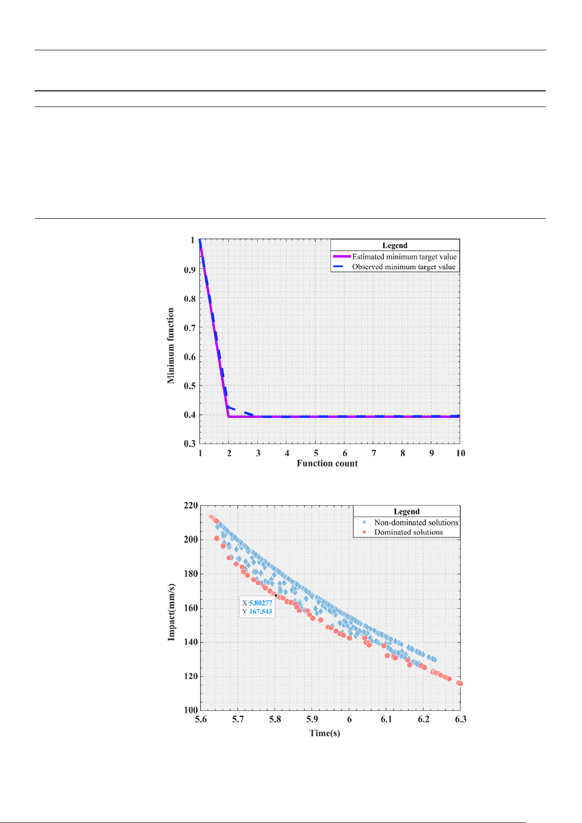
Figure 10. Function count.
Sensors2025,25,xFORPEERREVIEW 20 of 25
Figure10.Functioncount.
Figure11.Paretofrontier.
ToverifytheperformanceofBayesianoptimizationinoptimizingtheparametersof
theobjectivefunction,a5‐foldcross‐validationmethodwasadoptedinthisstudy.The
experimentalresultsareshowninFigure12.Itcanbeclearlyseenthattheperformance
ofthismodelduringthe5‐foldcross‐vali da tio n
processisrelativelystable,withasmall
fluctuationrangeoftheSingleScores,whichfullyindicatesthatthemodelhasacertain
fittingability.Generallyspeaking,across‐validationscorewithi n0.2canbere ga rd ed
asexcellent, andascorebetween0.2and0.5indicatesaverageperformance.Theaver‐
age
scoreofthisexperimentisapproximately0.4,whichindicatesthatthemodelhasa
certainpredictiveabilityonthisdatasetasa whole,butthereisstillroomforimprove‐
ment.
Figure 11. Pareto frontier.
Sensors 2025, 25, 1872
20 of 24
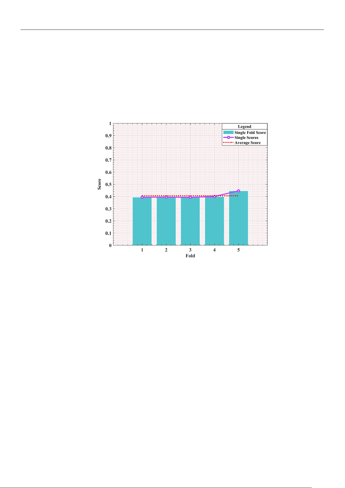
To verify the performance of Bayesian optimization in optimizing the parameters of
the objective function, a 5-fold cross-validation method was adopted in this study. The
experimental results are shown in Figure 12. It can be clearly seen that the performance
of this model during the 5-fold cross-validation process is relatively stable, with a small
fluctuation range of the Single Scores, which fully indicates that the model has a certain
fitting ability. Generally speaking, a cross-validation score within 0.2 can be regarded as
excellent, and a score between 0.2 and 0.5 indicates average performance. The average
score of this experiment is approximately 0.4, which indicates that the model has a certain
predictive ability on this dataset as a whole, but there is still room for improvement.
Sensors2025,25,xFORPEERREVIEW 21 of 25
Figure12.K‐FoldCrossValidationPerformance(K=5).
AccordingtothedataprovidedinTable10,Bayesianoptimizationisusedtoselect
thesecond‐generationsimulationresultswiththeminimumobjectivefunctionvalue.This
selection is based on minimization of the target value during the iteration. Figure 10.
clearly shows the dynamic change in the target value with the
iteration, making the
changeprocessclear. Fu rtheranalysisofFigure11, theminimumvalues ofF
1
andF
2
,
respectively,reach5.6294sand115.937mm/s.Andthetwominimumvaluesare,respec‐
tively,locatedatthetwoendsoftheParetofrontiercomposedofthereddots.Tooptimize
boththetimeandimpact,anoptimaladvantagemustbefoundontheParetofrontier.A
specificpoint
isidentifiedinFigure11 ,whichachievesanoptimalbalancebetweenthe
timeandimpact.Whena
max
andj
max
are78.1476mm/s
2
and119.8756mm/s
3
,thetimeand
impactoftheParetooptimalvalueare5.8028sand167.5427mm/s,respectively.
Usingthecomputeda
max
andj
max
,thesedataarereintegratedintothetrajectoryplan‐
ningoftheS‐shapedspeedcurve.Throughthisprocess,itispossibletoaccuratelydeter‐
minethepartialdisplacementofthetrajectoryplanninginthedirectionsoftheX‐axisand
Y‐axis,aswellastheassociatedcombinedvelocities,combined
accelerations,andcom‐
binedaccelerations,asshowninFigure13.Thesefiguresclearlyshowthattheplanned
S‐shapedspeedcurveexhibitedsmoothcharacteristicsduringmovement ,effectively
avoidingsuddenchangesandshocks.Thisisextremelyimportantforprecisionopera‐
tionssuchaswafer handling,asithelpsreducethedamage
thatcanbecausedbyimpact.
Table10.TheiterativegraphofBayesianthresholds.
Iteration Objective BestSoFar(Observed) BestSoFar(Estimated) Threshold
1
Threshold
2
Threshold
3
1 — — — 0.4227 0.7616 0.5225
2 0.3936 0.3936 0.4255 0.0989 0.7764 0.5705
3 0.3952 0.3936 0.3936 0.1721 0.7210 0.7933
4 0.3969 0.3936 0.3932 0.0752 0.4968 0.5437
5 0.3953 0.3936 0.3942 0.1403 0.6057 0.7633
6 0.3991 0.3936 0.3946 0.0500 0.5764 0.5441
7 0.3957 0.3936 0.3949 0.1485 0.5278 0.4003
8 0.3969 0.3936 0.3951 0.1113 0.7425 0.4637
9 0.3955
0.3936 0.3951 0.1592 0.7106 0.7313
10 0.3979 0.3936 0.3958 0.1587 0.6833 0.6341
Figure 12. K-Fold Cross Validation Performance (K = 5).
According to the data provided in Table 10, Bayesian optimization is used to select
the second-generation simulation results with the minimum objective function value. This
selection is based on minimization of the target value during the iteration. Figure 10. clearly
shows the dynamic change in the target value with the iteration, making the change process
clear. Further analysis of Figure 11, the minimum values of F
1
and F
2
, respectively, reach
5.6294 s and 115.937 mm/s. And the two minimum values are, respectively, located at the
two ends of the Pareto frontier composed of the red dots. To optimize both the time and
impact, an optimal advantage must be found on the Pareto frontier. A specific point is
identified in Figure 11, which achieves an optimal balance between the time and impact.
When a
max
and j
max
are 78.1476 mm/s
2
and 119.8756 mm/s
3
, the time and impact of the
Pareto optimal value are 5.8028 s and 167.5427 mm/s, respectively.
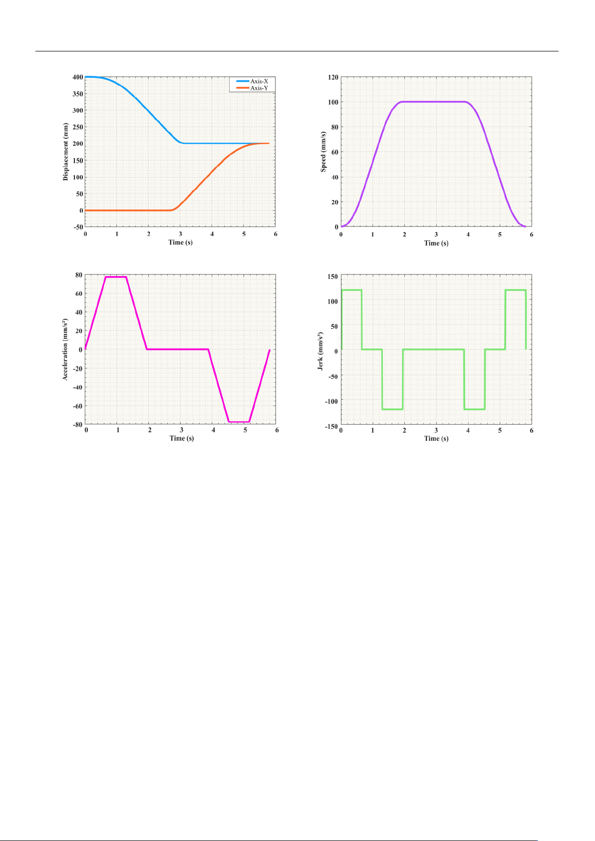
Using the computed a
max
and j
max
, these data are reintegrated into the trajectory planning
of the S-shaped speed curve. Through this process, it is possible to accurately determine the
partial displacement of the trajectory planning in the directions of the X-axis and Y-axis, as well
as the associated combined velocities, combined accelerations, and combined accelerations,
as shown in Figure 13. These figures clearly show that the planned S-shaped speed curve
exhibited smooth characteristics during movement, effectively avoiding sudden changes and
shocks. This is extremely important for precision operations such as wafer handling, as it
helps reduce the damage that can be caused by impact.
Sensors 2025, 25, 1872
21 of 24
Sensors2025,25,xFORPEERREVIEW 22 of 25
(a) (b)
(c) (d)
Figure13.Kinematicimage:(a)DisplacementcurveinCartesianspace;(b)speedcurveinCartes ian
space;(c)accelerationcurveinCartesianspace;(d)jerkcurveinCartesianspace.
Inaddition,thisstudymeticulouslyrecordsthekeyparameters,particularlythejoint
angles,duringtheS‐shapedspeedcurvemovement.Twosetsofjointanglesconsistingof
severalinterpolationpointsaresubstitutedintotheforwardkinematicsformula,asshown
inEquat ion(30).XandYrepr es ent thecoordi natevaluesinthe
Cartesiancoo r dinat e
system,respectively.
112 1 2
112 1 2
cos cos cos
sin sin sin
Xlink link
Y link link
(30)
TheactualmotiontrajectorydepictedintheplanarspaceisshowninFigure14.By
comparingFigures4and14,thehighconsistencyofthetwotrajectoriescanbecl earl y
verified.ThiscomparisonclearlyvalidatestheaccuracyandreliabilityoftheISO. This
planningmethodnotonlyelevatestheaccuracy
oftrajectoryplanning,butalsoensures
thesafetyandreliabilityofthemotion.
Figure 13. Kinematic image: (a) Displacement curve in Cartesian space; (b) speed curve in Cartesian
space; (c) acceleration curve in Cartesian space; (d) jerk curve in Cartesian space.
In addition, this study meticulously records the key parameters, particularly the joint
angles, during the S-shaped speed curve movement. Two sets of joint angles consisting of
several interpolation points are substituted into the forward kinematics formula, as shown
in Equation (30). X and Y represent the coordinate values in the Cartesian coordinate
system, respectively.
(
X = link
1
×cos θ
1
+ link
2
×
(
cos θ
1
+ cos θ
2
)
Y = link
1
×sin θ
1
+ link
2
×
(
sin θ
1
+ sin θ
2
)
(30)
The actual motion trajectory depicted in the planar space is shown in Figure 14. By
comparing Figures 4 and 14, the high consistency of the two trajectories can be clearly
verified. This comparison clearly validates the accuracy and reliability of the ISO. This
planning method not only elevates the accuracy of trajectory planning, but also ensures the
safety and reliability of the motion.