s25061872.pdf - 第14页
Sensors 2025 , 25 , 1872 14 of 24 3. Results 3.1. Ability T est and Analysis for ISO 3.1.1. Parameter Settings and Simulation Results In th is stu dy , all al gori thm ex per imen ts and si mul ati ons ar e per fo rmed u…
Sensors 2025, 25, 1872
13 of 24
but also provides theoretical support for the stable performance of the algorithm in un-
known scenarios.
2.4.5. ISO Algorithm Steps
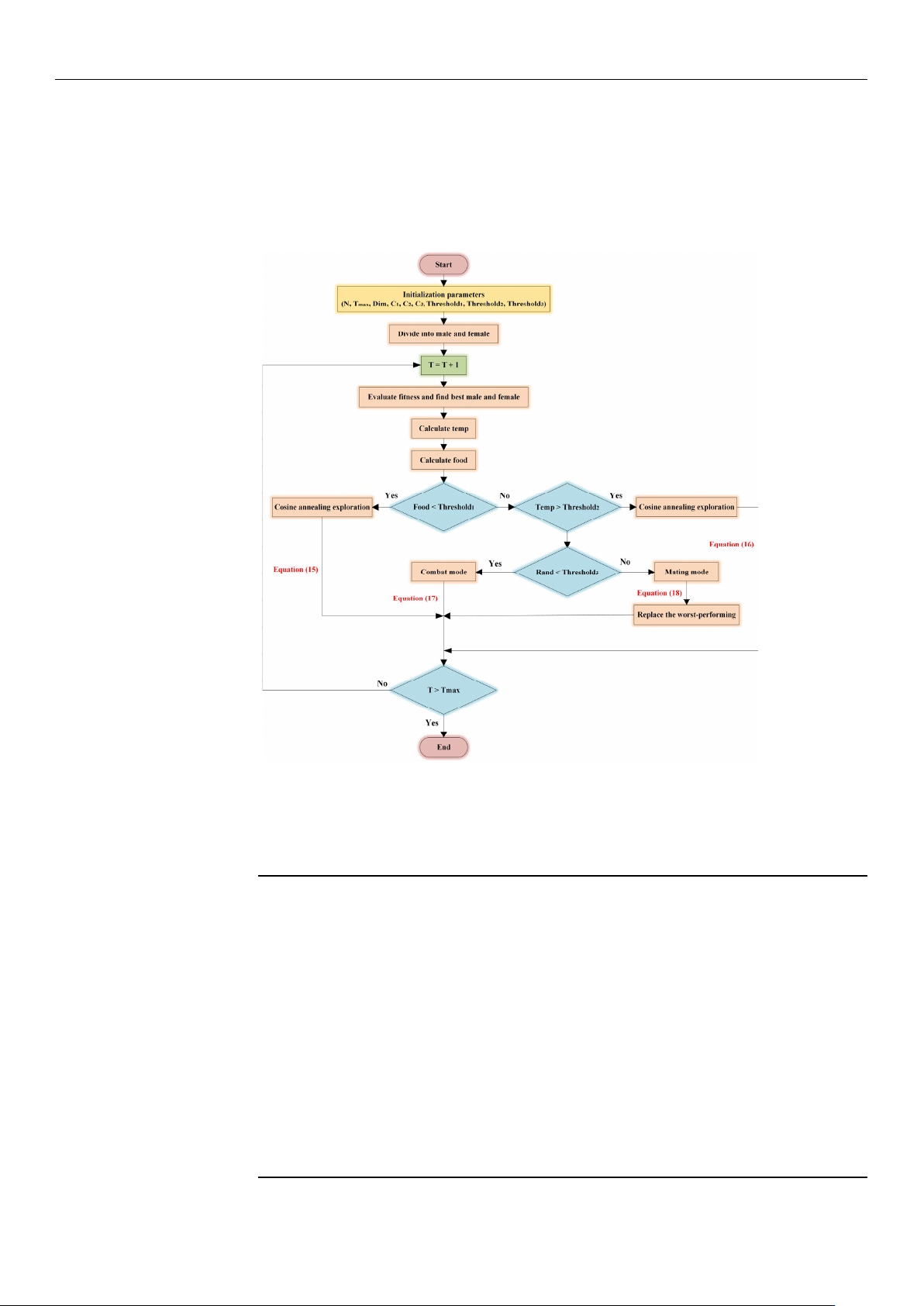
The flow chart of the ISO algorithm, which illustrates the step-by-step process, is
shown in Figure 8.
Sensors2025,25,xFORPEERREVIEW 14 of 25
Figure8.Theflowchartoftheimprovedsnakeoptimizationalgorithm.
TheISOalgorithmisoutlinedinAlgorithm,asshowninTable4.
Table4.ISOpseudo‐code.
1:Initializeparameters
2:InitializethepopulationusingtheTentChaoticMapasEquation(13)
3:DividepopulationintoN
mandNfusingEquations(10)and(11)
4:while(T<T
max)do
5:Evaluatethefitnessandidentifythebestfemaleandmale
6:CalculatetheiterationtemperatureandfoodquantityEquation(14)
7:if(Food<threshold
1)then
8:CosineannealingexplorationusingEquation(15)
9:elseif(Temp>threshold
2)then
10:CosineannealingexplorationusingEquation(16)
11:else
12:if(rand<threshold
3)then
13:EnterFightModeusingEquation(17)
14:else
15:EnterMatingModeusingEquation(18)
16:Replacetheworst‐performingfemaleandmale
Figure 8. The flow chart of the improved snake optimization algorithm.
The ISO algorithm is outlined in Algorithm, as shown in Table 4.
Table 4. ISO pseudo-code.
1: Initialize parameters
2: Initialize the population using the Tent Chaotic Map as Equation (13)
3: Divide population into N
m
and N
f
using Equations (10) and (11)
4: while (T < T
max
) do
5: Evaluate the fitness and identify the best female and male
6: Calculate the iteration temperature and food quantity Equation (14)
7: if (Food < threshold
1
) then
8: Cosine annealing exploration using Equation (15)
9: else if (Temp > threshold
2
) then
10: Cosine annealing exploration using Equation (16)
11: else
12: if (rand < threshold
3
) then
13: Enter Fight Mode using Equation (17)
14: else
15: Enter Mating Mode using Equation (18)
16: Replace the worst-performing female and male
17: end if
18: end if
19: end while
20: Return the optimal solution

Sensors 2025, 25, 1872
14 of 24
3. Results
3.1. Ability Test and Analysis for ISO
3.1.1. Parameter Settings and Simulation Results
In this study, all algorithm experiments and simulations are performed using MAT-
LAB 2022B software platform. To verify the convergence performance and accuracy of
the ISO algorithm, five heuristic algorithms—SO [
40
], SA [
41
], PSO [
19
], GWO [
42
], and
WOA
[43]—are
added for comparison. In addition, to ensure the rigor and accuracy of the
experimental results, the CEC2005 benchmark test set is selected as the objective function, as
listed in Table 5. Five unimodal functions (F
1
–F
5
) and three multi-modal functions (F
6
–F
8
) are
listed in Table 5. Through an in-depth analysis of these benchmark functions, the performance
of the ISO algorithm is evaluated to a certain extent.
Table 5. Test functions.
Function Range Min
F
1
(x) =
n
∑
i=1
x
2
i
[−100,100] 0
F
2
(x) =
n
∑
i=1
|
x
i
|
+
n
∏
i=1
|
x
i
|
[−10,10] 0
F
3
(x) =
n
∑
i=1
i
∑
j=1
x
j
!
2
[−100,100] 0
F
4
(x) = max
i
{|
x
i
|
, 1 ≤ i ≤ n
}
[−100,100] 0
F
5
(x) =
n
∑
i=1
ix
4
i
+ randm[0, 1)
[−128,128] 0
F
6
(x) =
n
∑
i=1
(x
2
i
−10 cos(2πx
i
) + 10)
[−5.12,5.12] 0
F
7
(x) =
1
4000
d
∑
i=1
x
2
i
−
d
∏
i=1
cos(
x
i
√
i
) + 1
[−600,600] 0
F
8
(x) =0.1
sin
2
(3πx
1
) +
n
∑
i=1
(x
i
−1)
2
1 + sin
2
(3πx
i
+ 1)
+ (x
n
−1)
2
1 + sin
2
(2πx
n
)
+
n
∑
i=1
u(x
i
, 5, 100, 4),
u(x
i
, a, k, m) =
k(x
i
− a)
m
, x
i
> a
0, a > x
i
> −a
k(−x
i
− a)
m
, x
i
< −a
[−50,50] 0
Before simulating the benchmark test functions for the six heuristic algorithms, a brief
introduction to their main parameter settings is necessary to ensure that researchers can
obtain similar experimental results when conducting simulations. To ensure the fairness of
experiments, the population size (N) of all algorithms is set to 50, the maximum iteration
number (T
max
) is set to 100, the dimension (Dim) is set to 30, and each algorithm is run
20 times independently. For the other key parameters within the algorithms, recommended
values based on experience are used for setting, and the specific parameter values are listed
in Table 6. After successfully configuring these parameters, a MATLAB script is used to
start the six algorithms simultaneously. The experimental results are summarized in Table 7,
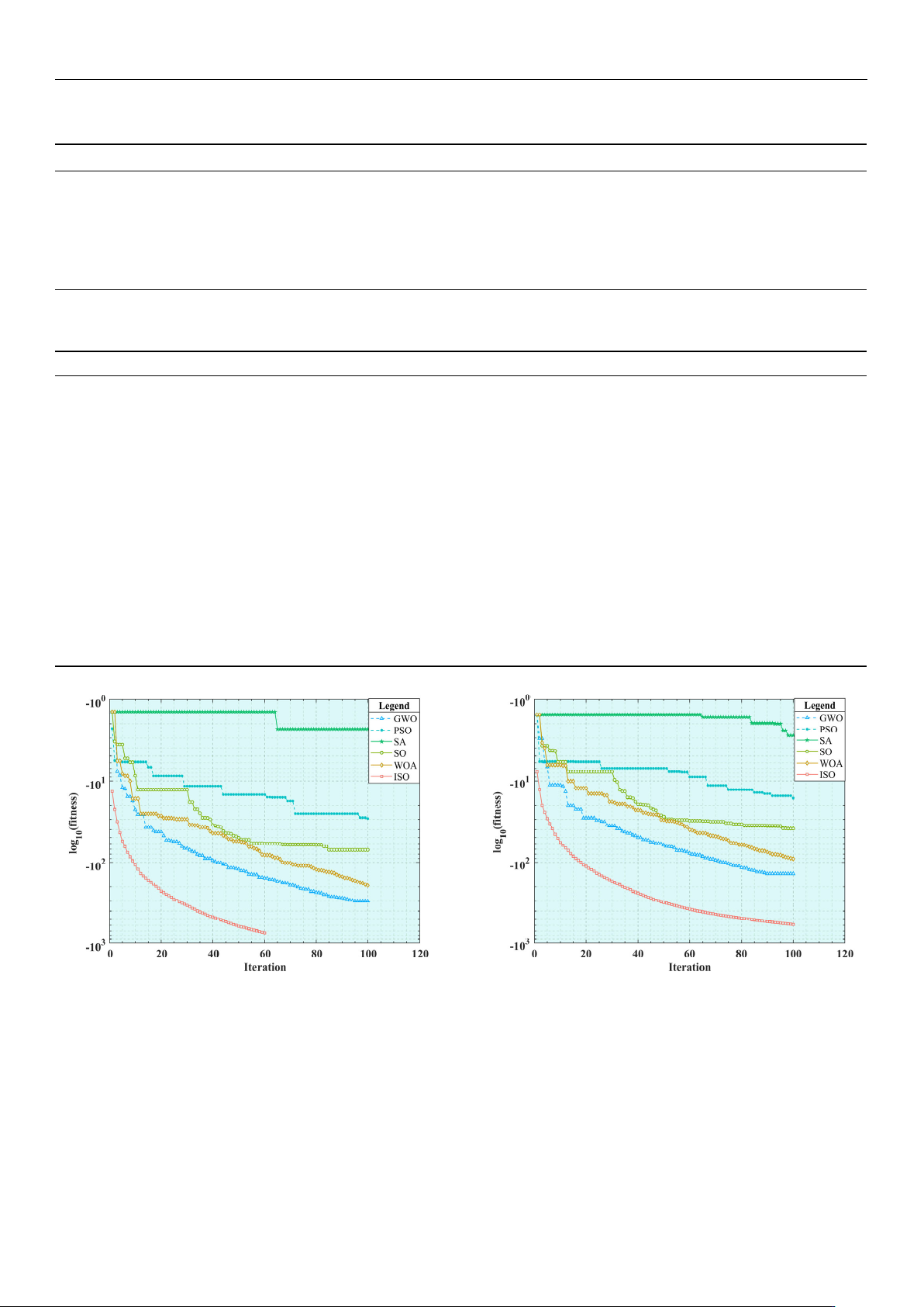
and the iteration curves of the benchmark test functions are displayed in Figure 9.
Sensors 2025, 25, 1872
15 of 24
Table 6. Parameter settings for the algorithms.
Algorithm Parameter Settings
SO Theshold
1
= 0.25, Theshold
2
= 0.6, Theshold
3
= 0.6, C
1
= 0.5, C
2
= 0.05, C
3
= 2
SA Temp = 100, Temp
min
= 0.01, alpha = 0.95
PSO w = 0.9, c
1
= 2, c
2
= 2, V
max
= 0.3 ∗ ub, V
min
= 0.3 ∗ lb
GWO r
1
= r
2
= rand
WOA r
1
= r
2
= rand, p = rand, b = 1
ISO sigma = 0.1, alpha
min
= 0.01, alpha
max
= 1.0, eta
max
= 0.01, eta
min
= 0.001
Table 7. Results obtained by different algorithms (D = 30).
Function SO SA PSO GWO WOA ISO
F
1
MEAN
8.27 × 10
−40
7.30 × 10
−2
3.04 × 10
−12
6.24 × 10
−105
8.40 × 10
−79
0
STD
2.51 × 10
−39
2.27 × 10
−1
6.51 × 10
−12
2.79 × 10
−104
2.10 × 10
−78
0
F
2
MEAN
3.95 × 10
−21
4.26 × 10
−2
1.38 × 10
−7
8.55 × 10
−57
2.95 × 10
−40
9.14 × 10
−214
STD
5.26 × 10
−21
2.87 × 10
−2
2.22 × 10
−7
3.13 × 10
−56
7.95 × 10
−40
0
F
3
MEAN
2.16 × 10
−39
3.85 × 10
−2
6.47 × 10
−12
6.66 × 10
−107
2.18 × 10
−79
0
STD
7.04 × 10
−39
8.37 × 10
−2
2.16 × 10
−11
2.98 × 10
−106
6.74 × 10
−79
0
F
4
MEAN
2.01 × 10
−20
1.34 × 10
−1
1.38 × 10
−6
1.27 × 10
−53
8.56 × 10
−40
2.27 × 10
−213
STD
3.54 × 10
−20
9.71 × 10
−2
2.36 × 10
−6
3.93 × 10
−53
2.64 × 10
−39
0
F
5
MEAN
7.01 × 10
−4
6.64 × 10
−1
1.77 × 10
−3
5.21 × 10
−4
7.33 × 10
−4
1.75 × 10
−4
STD
7.23 × 10
−4
8.91 × 10
−1
1.26 × 10
−3
5.08 × 10
−4
7.05 × 10
−4
2.72 × 10
−4
F
6
MEAN 0
1.79 × 10
−2
2.39 × 10
−12
0 0 0
STD 0
3.42 × 10
−2
3.35 × 10
−12
0 0 0
F
7
MEAN 0
1.67 × 10
−2
6.15 × 10
−12
0 0 0
STD 0
3.42 × 10
−2
3.35 × 10
−12
0 0 0
F
8
MEAN
1.74 × 10
1
1.10 × 10
9
4.41 × 10
1
1.24 × 10
0
8.13 × 10
−1
2.06 × 10
−1
STD
3.32 × 10
1
1.35 × 10
8
2.59 × 10
1
4.26 × 10
−1
3.08 × 10
−1
2.03 × 10
−1
Sensors2025,25,xFORPEERREVIEW 16 of 25
222 22
81
1
1
( ) 0.1 sin (3 ) ( 1) 1 sin (3 1) ( 1) 1 sin ( 2 )
( ,5,100, 4),
(),
(,,,) 0,
(),
n
iin n
i
n
i
i
m
ii
ii
m
ii
Fx x x x x x
ux
kx a x a
ux akm a x a
kxa x a
[−50,50] 0
Table6.Parameterseingsforthealgorithms.
Algorithm ParameterSeings
SO Theshold1=0.25,Theshold2=0.6,Theshold3=0.6,C1=0.5,C2=0.05,C3=2
SA Temp=100,Tempmin=0.01,alpha=0.95
PSO w=0.9,c
1=2,c2=2,Vmax=0.3*ub,Vmin=0.3*lb
GWO r
1=r2=rand
WOA r
1=r2=rand,p=rand,b=1
ISO sigma=0.1,alpha
min=0.01,alphamax=1.0,etamax=0.01,etamin=0.001
Table7.Resultsobtainedbydifferentalgorithms(D=30).
Function SO SA PSO GWO WOA ISO
F1
MEAN 8.27×10
−40
7.30×10
−2
3.04×10
−12
6.24×10
−105
8.40×10
−79
0
STD 2.51×10
−39
2.27×10
−1
6.51×10
−12
2.79×10
−104
2.10×10
−78
0
F
2
MEAN 3.95×10
−21
4.26×10
−2
1.38×10
−7
8.55×10
−57
2.95×10
−40
9.14×10
−214
STD 5.26×10
−21
2.87×10
−2
2.22×10
−7
3.13×10
−56
7.95×10
−40
0
F
3
MEAN 2.16×10
−39
3.85×10
−2
6.47×10
−12
6.66×10
−107
2.18×10
−79
0
STD 7.04×10
−39
8.37×10
−2
2.16×10
−11
2.98×10
−106
6.74×10
−79
0
F
4
MEAN 2.01×10
−20
1.34×10
−1
1.38×10
−6
1.27×10
−53
8.56×10
−40
2.27×10
−213
STD 3.54×10
−20
9.71×10
−2
2.36×10
−6
3.93×10
−53
2.64×10
−39
0
F
5
MEAN 7.01×10
−4
6.64×10
−1
1.77×10
−3
5.21×10
−4
7.33×10
−4
1.75×10
−4
STD 7.23×10
−4
8.91×10
−1
1.26×10
−3
5.08×10
−4
7.05×10
−4
2.72×10
−4
F
6
MEAN 0 1.79×10
−2
2.39×10
−12
0 0 0
STD 0 3.42×10
−2
3.35×10
−12
0 0 0
F
7
MEAN 0 1.67×10
−2
6.15×10
−12
0 0 0
STD 0 3.42×10
−2
3.35×10
−12
0 0 0
F
8
MEAN 1.74×10
1
1.10×10
9
4.41×10
1
1.24×10
0
8.13×10
−1
2.06×10
−1
STD 3.32×10
1
1.35×10
8
2.59×10
1
4.26×10
−1
3.08×10
−1
2.03×10
−1
(a) (b)
Figure 9. Cont.