s25061872.pdf - 第9页
Sensors 2025 , 25 , 1872 9 of 24 si ti on of th is in it ia l p op ul at io n c an be r ep r es en te d b y E qu at io n ( 6) , w he r e t he nu mb er s of ma le an d fe ma le in di vi du al s a r e r e p r es en te d b …
Sensors 2025, 25, 1872
8 of 24
By analyzing the data in Table 2, it is clear that this trajectory planning task involves
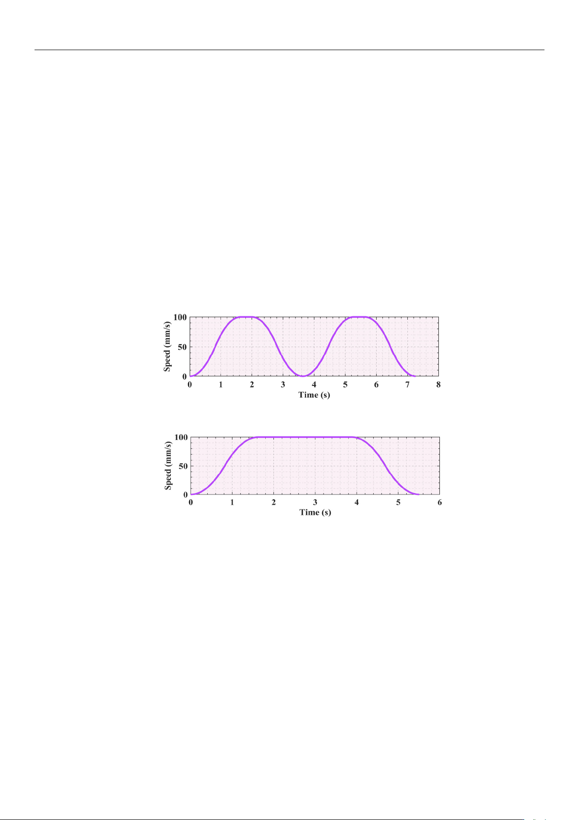
three key nodes that the robotic arm must reach in sequence. S-shaped speed curve planning
is a standard point-to-point start–stop motion scheme. Specifically, this task is represented
by two movements from the starting point to the middle point and then from the middle
point to the end point, with zero starting and ending speeds for each movement. Based
on the data in Table 3, the velocity image of the scheme is shown in Figure 5. However,
this scheme causes the manipulator to frequently start and stop, which not only increases
the vibration during the motion process but also leads to time wastage in the acceleration
and deceleration stages. To address this issue, an improved scheme is proposed in this
study for the single-segment start–stop mechanism, optimizing the starting and stopping
parts of the intermediate process into a smooth motion mode with constant speeds at both
ends, as shown in Figure 6. When the velocity of the first segment of motion attains the
maximum value of the set parameters, instead of reducing the velocity back to zero as in the
standard scheme, the second segment of motion proceeds in a uniform transition manner.
The specific parameters still refer to Table 3. This improved scheme effectively mitigates the
limitations inherent in the conventional approach. Simultaneously, the movement efficiency
can be improved and the vibration can be reduced.
Sensors2025,25,xFORPEERREVIEW 8 of 25
transitioncanbeadjustedaccordingtospecificworkrequirements.Overall,thecircular
transitionnotonlyimprovesthesmoothnessandefficiencyoftheroboti carm’smotion
but also helpstoprotectthe roboticarmandits payload, whileenhancing the overall
operational performance. This transition method allows the robotic arm
to pe rf or m
complextasksmoreaccuratelyandreliably.
Figure4.Contrastdiagramofarctransitionandright‐anglepath.
ByanalyzingthedatainTable2,itisclearthatthistrajectoryplanningtaskinvolves
threekeynodesthattheroboticarmmustreachinsequence.S‐shapedspeedcurve
planningisastandardpoint‐to‐pointstart–stopmotionscheme.Specifically,thistaskis
representedbytwomovementsfrom
thestartingpointtothemiddlepoint andthen
fromthemiddlepointtotheendpoint,withzerostartingandendingspeedsforeach
movement.BasedonthedatainTable3,thevelocityimageoftheschemeisshownin
Figure5.However,thisschemecausesthemanipulator
tofrequentlystartandstop,which
notonlyincreasesthevibrationduringthemotionprocessbutalsoleadstotimewastage
intheaccelerationanddecelerationstages.Toaddressthisissue,animprovedschemeis
proposed in this study for the single‐segment start–st op mechanism, optimizing the
startingandstoppingparts
oftheintermediateprocessintoasmoothmotionmodewith
constantspeedsatbothends,asshowninFigure6.Whenthevelocityofthefirstsegment
ofmotionattainsthemaximumva lueofthesetparameters,insteadof reducingthe
velocitybacktozeroasinthestandardscheme,
thesecondsegmentofmotionproceeds
inauniformtransitionmanner.Thespecificpara mete rsstillrefertoTable 3.This
improved scheme effectively mitigates the limitations inherent in the conventiona l
approach.Simultaneously,themovementefficiencycanbeimprovedand thevi bra ‐
tioncanbereduced.
Figure5.Thecontinuousstart–stopS‐shapedspeedcurve.
Figure 5. The continuous start–stop S-shaped speed curve.
Sensors2025,25,xFORPEERREVIEW 9 of 25
Figure6.Theimprovedstart–stopS‐shapedspeedcurve.
ComparingFigures5and6,itcanbeseenthattheimprovedmotionschemeresults
inasmootherspeedcurve.Concurrently,iteffectivelyreducesthevibrationgenerated
bythemot orduringstarting andstopping.Wit hthebasic para metersunchanged,
theunoptimized timeschedulewhich doesnot include arcadjustment and smooth
transitiontook7.26s,whereas theoptimizedtimeschedule, whichincludesarcadjust‐
mentandsmoothtransition,isshortenedto5.51s.Afterthetwopartsareoptimized,the
totaltimeissavedby1.75s,a24.1%reductioncomparedtotheoriginalscheme.
2.4.ImprovedSnakeOptimizationAlgorithm
2.4.1.
InitializationPopulationofaTentChaoticMap
Thesnakeoptimization(SO)algorithmisanintelligentoptimizationtechniquethat
simulatesthespecificmatingbehaviorofsnakes.Itachievesaneffectivebalancebetween
globalandlocalsearchesbyusingauniquesearchmechanism.Intheinitializationphase
ofthealgorithm,individuals
inthepopulationareequallydividedintomaleandfemale
individuals.ThecompositionofthisinitialpopulationcanberepresentedbyEquation(6),
wherethenumbersofmaleandfemaleindividualsarerepresentedbyEquations(7)and
(8),respectively.
()
i
X
lb rand ub lb
(6)
2
m
N
N
(7)
f
m
NNN
(8)
whereX
idenotesthepositionofthei‐thindividual.Therandomfunction‘rand’generates
arealrandomnumberbetween0and1.TheupperandlowerboundsofXiareubandlb,
respectively.N isthetotalpopulationsize. N
m andNfare the numbers of individual
malesandfemales,respectively.
However,theuseofthefunction‘rand’inEquation(6)oftheSOalgorithmmayresult
inanunevendistributionofrandomnumbers.Moreover,becausethisfunctionisbased
onadeterministicalgorithm,thesamerandomsequenceisgeneratedwhen
thesameseed
isgiven.Thissituationmayleadtotheprematureconvergenceoftheheuristicalgorithm
tothelocaloptimalsolution,makingitchallengingtofindtheglobaloptimalsolution.To
addressthisissueinpopulationinitialization,thisstudyintroducesaTentChaoticMap.
Ithas excellentchaoticcharacteristics,
whichcaneffectivelyimprove the uniformityof
population distri buti on. In addition, co mpa re d with Sine and Logistic chaotic map
[32,33],itsimplementationismore intuitiveandsimple,whileSineandLogisticchaotic
map’slatedepthsearchabilityisweak,whichmaycausethealgorithmtofallinto local
optimal. At the
same time, thedistributi o n of theiroutput sequencemay be uneven
undercertainpa ra m etervalues.Asaconsequence,theTentChaosmapisagoodchoice
Figure 6. The improved start–stop S-shaped speed curve.
Comparing Figures 5 and 6, it can be seen that the improved motion scheme results
in a smoother speed curve. Concurrently, it effectively reduces the vibration generated
by the motor during starting and stopping. With the basic parameters unchanged, the
unoptimized time schedule which does not include arc adjustment and smooth transition
took 7.26 s, whereas the optimized time schedule, which includes arc adjustment and
smooth transition, is shortened to 5.51 s. After the two parts are optimized, the total time is
saved by 1.75 s, a 24.1% reduction compared to the original scheme.
2.4. Improved Snake Optimization Algorithm
2.4.1. Initialization Population of a Tent Chaotic Map
The snake optimization (SO) algorithm is an intelligent optimization technique that simu-
lates the specific mating behavior of snakes. It achieves an effective balance between global and
local searches by using a unique search mechanism. In the initialization phase of the algorithm,
individuals in the population are equally divided into male and female individuals. The compo-

Sensors 2025, 25, 1872
9 of 24
sition of this initial population can be represented by Equation (6), where the numbers of male
and female individuals are represented by Equations (7) and (8), respectively.
X
i
= lb + rand ×(ub −lb) (6)
N
m
=
N
2
(7)
N
f
= N − N
m
(8)
where X
i
denotes the position of the i-th individual. The random function ‘rand’ generates
a real random number between 0 and 1. The upper and lower bounds of X
i
are ub and lb,
respectively. N is the total population size. N
m
and N
f
are the numbers of individual males
and females, respectively.
However, the use of the function ‘rand’ in Equation (6) of the SO algorithm may result
in an uneven distribution of random numbers. Moreover, because this function is based on
a deterministic algorithm, the same random sequence is generated when the same seed is
given. This situation may lead to the premature convergence of the heuristic algorithm to
the local optimal solution, making it challenging to find the global optimal solution. To
address this issue in population initialization, this study introduces a Tent Chaotic Map.
It has excellent chaotic characteristics, which can effectively improve the uniformity of
population distribution. In addition, compared with Sine and Logistic chaotic map [
32
,
33
],
its implementation is more intuitive and simple, while Sine and Logistic chaotic map’s
late depth search ability is weak, which may cause the algorithm to fall into local optimal.
At the same time, the distribution of their output sequence may be uneven under certain
parameter values. As a consequence, the Tent Chaos map is a good choice in this study.
And the Tent Chaos Map can be expressed as Equation (9). And ‘x
i
’ replaces ‘rand’ as shown
in Equation (10).
x
i+1
=
x
i
a
, 0 ≤ x
i
< a
1−x
i
1−a
, a ≤ x
i
≤ 1
(9)
X
i
= lb + x
i
×(ub −lb) (10)
where x
i
and x
i+
1
stand for the i-th and i + 1-th values of Tent Chaotic Map, respectively. X
i
stands for the i-th individual position. Moreover, parameter a is the variable value, which
is 0.5 in this study [34].
2.4.2. Dynamic Learning Factor with Random Noise
In heuristic algorithms, learning factors play a key role in regulating the search be-
havior, including the balance between exploration and exploitation. Exploration refers
to the ability to search for new solutions randomly, whereas development refers to the
ability to search locally for the best solution. The learning factors of the SO algorithm
include the constant value C
1
of the food calculation equation, constant value C
2
of the
food exploration stage, and constant value C
3
of the food development stage. The initial
values of these constants are typically set to C
1
= 0.5, C
2
= 0.05, and C
3
= 2. The equations
containing C
1
, C
2
, and C
3
are Equations (11)–(15). The subscript ‘m’ and ‘f ’ refers to the
male and female snakes, respectively. The special mention of female snake expressions will
be omitted in the following text.
Q = C
1
×(
t − T
T
) (11)
X
i, m_1
(t + 1) = X
rand, m_1
(t) ±C
2
× A
m
×
[
(ub − lb) ×rand + lb
]
(12)

Sensors 2025, 25, 1872
10 of 24
X
i, m_2
(t + 1) = X
food
(t) ±C
3
×Temp ×rand ×
[
X
food
(t) − X
i, m
(t)
]
(13)
X
i, m_3
(t + 1) = X
i, m_3
(t) ±C
3
× F
m
×rand ×
h
Q × X
best, f
− X
i, m
(t)
i
(14)
X
i, m_4
(t + 1) = X
i, m_4
(t) ±C
3
× M
m
×rand ×
h
Q × X
i, f
(t) − X
i, m
(t)
i
(15)
where Q is the amount of food consumed. t denotes the current number of itera-
tions. T denotes the maximum number of iterations. Temp is the iteration temperature.
X
i
, m_1
, X
i
, m_
2
, X
i
, m_3
,
and X
i
, m_4
are the locations of food in the exploration phase of male
snakes, food in the development phase of male snakes, combat mode in the development
phase of male snakes, and mating mode in the development phase of male snakes, respec-
tively. X
rand
, m_1
is the randomly selected male population. X
best_f
is the best position for
the females in this population. A
m
, F
m
, and M
m
are measured for the male’s ability to find
food, the male’s ability to fight, and the male’s ability to mate.
Because the learning factors C
1
, C
2
, and C
3
remain unchanged during the iteration, the
algorithm may not adapt to the dynamic changes in the solution space. Hence, the delta
value is introduced for the normal distribution of random tubs. This perturbation helps
the SO algorithm eliminate the trap of local optimal solutions, thus enhancing its global
search abilities. In addition, the literature [
35
] introduces a learning strategy employed
within the ISO framework, which centers on acquiring knowledge from the experiences
of other group members. This approach aims to mitigate the likelihood of converging on
local optima. Nonetheless, the implementation of such specialized learning mechanisms
not only entails a notable increase in algorithmic complexity but also exhibits diminished
efficacy when adapting to the diverse phases of the optimization procedure. However, the
SO algorithm can achieve an effective dynamic balance between global and local searches
by dynamically adjusting these fixed learning factors C
1
, C
2
, and C
3
, thereby improving
the performance and efficiency of the algorithm. The concrete expression of the random
disturbance is shown in Equations (16) and (17). In Equation (19), alpha is used to store the
parameter values for learning factors C
1
, C
2
, and C
3
.
delta = sigma ×randn (16)
al pha(t + 1) = alpha(t) + delta (17)
where sigma represents the amplitude of the perturbation. It is 0.1 in this paper [
36
]. alpha is
limited to a range between 0.01 and 1. Random function ‘randn’ represents a random value
with a standard normal distribution.
2.4.3. Cosine Annealing Learning Rate
In Equations (12)–(15), the strategy for updating the individual positions is relatively
simple. Without considering adjusting the strategy as an iteration progress, the SO algo-
rithm mainly relies on the current individual’s position and velocity vector to determine
the next individual’s position. This method is more likely to cause the algorithm to become
stuck in a locally optimal solution. To improve the update strategy of the original SO
algorithm, this study introduced a cosine learning annealing rate. This strategy simulates
the dynamic adjustment of the learning rate based on the cosine function, which can dy-
namically adjust the speed of the position updating based on the number of iterations. In
the early stages of the iteration, the learning rate can be reduced rapidly to achieve fast
convergence. In the later stages of the iteration, fine adjustments are made to optimize the
precision of the solution by reducing the learning rate, as shown in Figure 7. The specific
expression of the cosine learning annealing rate is shown in Equation (18).