mi17050592.pdf - 第12页

Micromachines 2026 , 17 , 592 12 of 34 into the photonic integrated cir cuit via an input grating coupler , propagates through a dedicated on-die optical loopback waveguide, and is subsequently extracted thr ough an adja…

Micromachines 2026, 17, 592

11 of 34

3.2. Experimental Characterization

3.2.1. Hysteresis Measurement

As described in Section 2, the piezoelectric actuators in the Eclipse Dynamic system

exhibit path-dependent hysteresis whose magnitude scales with the applied voltage range.

To quantify this behavior for the speciﬁc axes and operating conditions of this work, we

performed controlled voltage sweeps on the physical hardware while measuring displace-

ment with a high-resolution optical measurement system. A ceramic reference plate with

precision markers was mounted on the ﬂexure, and displacement was recorded as voltage

was increased and decreased in steps.

The experimental protocol reads as follows. Voltage was swept for each of the three

physical actuators (X, Y1, and Y2) from 0 V to each of six peak levels (20, 40, 60, 80, 100,

and 120 V) and returned to 0 V, with the resulting spatial displacement recorded at every

step. This protocol isolates how hysteresis error scales with the peak operating voltage.

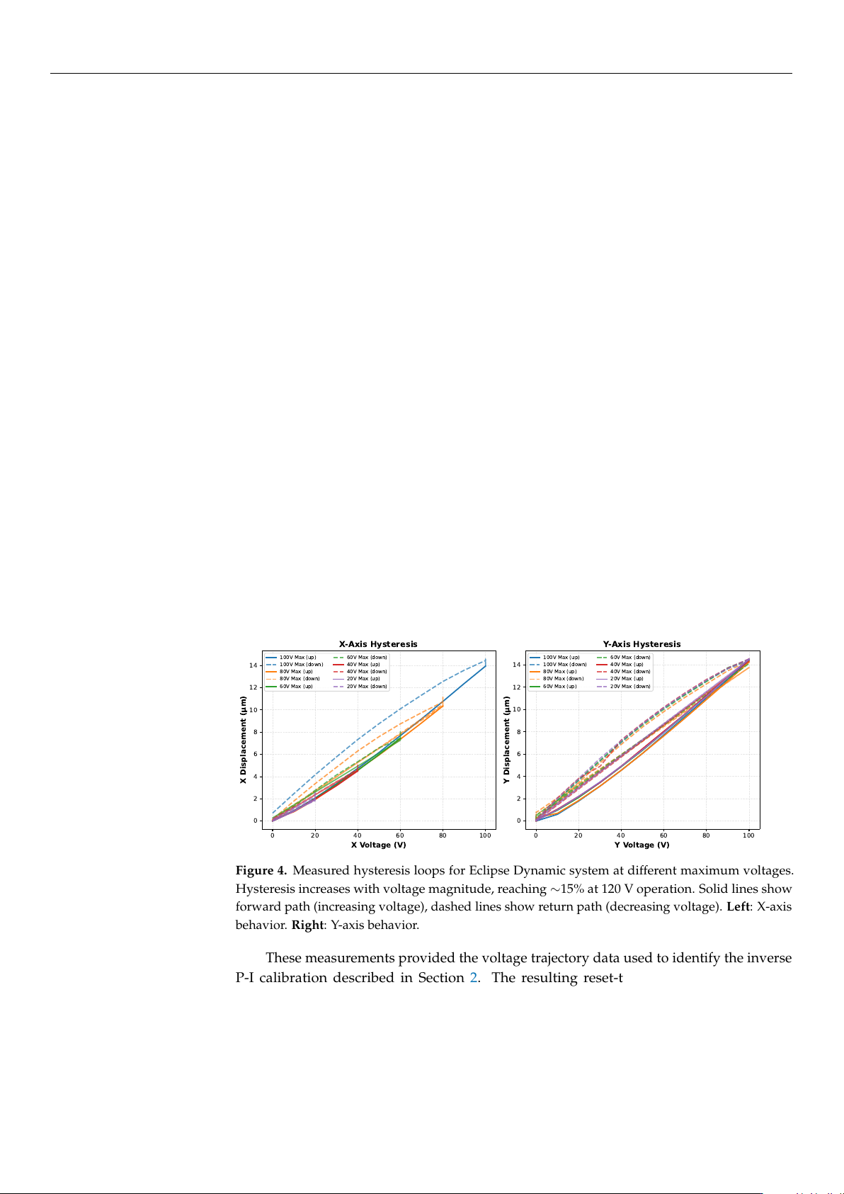
The measured hysteresis loops representing the resulting spatial movement along

the X and Y axes are shown in Figure 4. Three characteristics are directly relevant to the

algorithm design. First, hysteresis is strongly voltage-dependent: at a peak drive of 100 V

the X-axis positioning error is approximately 3.5%, whereas extending to the full 120 V

operating range raises this to approximately 15%. Second, the forward path (increasing

voltage, solid lines) and return path (decreasing voltage, dashed lines) diverge substantially,

with the descending trajectory consistently underreaching the forward-path displacement

at equivalent drive levels. Third, restricting actuation to the 20–40 V range limits hysteresis

to 2–4%, indicating that algorithms operating via small, localized voltage increments will

inherently encounter fewer nonlinearity effects than those requiring wide-range excursions.

We additionally observed a slight non-orthogonality between the X and Y axes, attributed

to asymmetric Y1/Y2 actuator characteristics and their sequential rather than simultaneous

activation; this cross-coupling is accounted for in all alignment algorithm implementations.

0 20 40 60 80 100

X Voltage (V)

X Displacement ( m)

X-Axis Hysteresis

100V Max (up)

100V Max (down)

80V Max (up)

80V Max (down)

60V Max (up)

60V Max (down)

40V Max (up)

40V Max (down)

20V Max (up)

20V Max (down)

0 20 40 60 80 100

Y Voltage (V)

Y Displacement ( m)

Y-Axis Hysteresis

100V Max (up)

100V Max (down)

80V Max (up)

80V Max (down)

60V Max (up)

60V Max (down)

40V Max (up)

40V Max (down)

20V Max (up)

20V Max (down)

Figure 4. Measured hysteresis loops for Eclipse Dynamic system at different maximum voltages.

Hysteresis increases with voltage magnitude, reaching

∼

15% at 120 V operation. Solid lines show

forward path (increasing voltage), dashed lines show return path (decreasing voltage). Left: X-axis

behavior. Right: Y-axis behavior.

These measurements provided the voltage trajectory data used to identify the inverse

P-I calibration described in Section 2. The resulting reset-to-zero timing overhead is

captured in the hardware timing model of Section 3.3.4.

3.2.2. Optical Power Measurements

The experimental optical setup is conﬁgured to measure insertion loss continuously

during the active alignment process. The apparatus utilizes a continuous-wave laser source

coupled into the single-mode optical ﬁbers of the integrated probe head. Light is injected

https://doi.org/10.3390/mi17050592

Micromachines 2026, 17, 592

12 of 34

into the photonic integrated circuit via an input grating coupler, propagates through a

dedicated on-die optical loopback waveguide, and is subsequently extracted through an

adjacent output grating coupler. The transmitted optical signal is collected by a return ﬁber

within the array and recorded by a high-speed optical power meter. This continuous data

stream provides the real-time optical power feedback required by the control software to

evaluate coupling efﬁciency and direct the piezoelectric actuators.

Utilizing this loopback conﬁguration, eight distinct experimental alignment campaigns

were conducted across various grating coupler positions and individual dies. This exper-

imental design comprehensively captures the variability arising from die-to-die process

ﬂuctuations and position-dependent spatial non-uniformities across the wafer. Further-

more, repeated measurements on a single die provide critical insight into overall system

repeatability and environmental stability. Each experimental campaign thus serves as

a highly realistic test case for evaluating algorithm robustness under authentic produc-

tion conditions.

The initial physical measurements were executed using baseline algorithm param-

eters. During this phase, the BO algorithms employed conservative settings: the Global

Bayesian method used 8 initial Latin-Hypercube sampled points [

] and a maximum of

70 iterations, while gradient-based methods used moderate, non-adaptive step sizes and

learning rates. These initial parameters, while functional, were not yet optimized for the

speciﬁc characteristics of the Eclipse Dynamic system or the optical coupling landscape

topology observed in practice. The experimental results presented in Section 4 therefore

reﬂect this initial algorithm conﬁguration.

In the updated version of the alignment algorithms used for the comprehensive

simulation study, the methods were reﬁned to maximize both efﬁciency and reliability.

Speciﬁcally, the gradient-based approaches were upgraded with adaptive step sizes and

ﬁner convergence logic to better leverage the system 1 nm hardware positioning resolu-

tion. All detailed mathematical parameters and control logic for these reﬁned algorithms,

including the speciﬁc adaptive formulations, are fully explained in Section 3.4. The sim-

ulation framework and the deﬁnitive results reported in Section 4 employ these reﬁned,

production-ready conﬁgurations. By testing these optimized algorithms across 72 unique

spatial windows representing a 9

increase in scenario diversity compared to the initial

experiments, we established the ﬁnal performance rankings and recommendations for

high-volume PIC manufacturing.

3.3. Simulation Framework

To enable systematic evaluation across a wider range of conditions, we developed a

simulation framework that generates synthetic alignment scenarios from experimental data.

The objective is to validate algorithm performance without requiring physical hardware

by creating high-resolution ground-truth surfaces from discrete measurement data, and

generating mock data ﬁles that mimic the limited ﬁeld of view of the hardware during

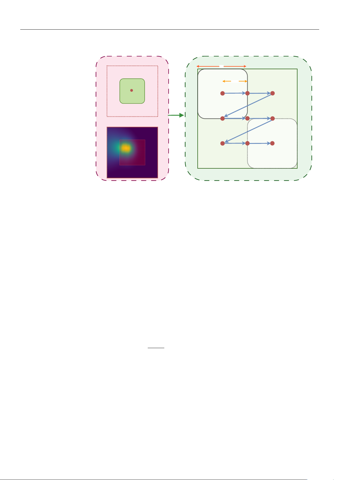
operation. Figure 5 summarizes the simulation pipeline used in this work. Starting from

each experimental scan, we reconstruct a continuous ground-truth coupling surface via

Radial Basis Function (RBF) interpolation, to establish an extrapolated 240 V

240 V virtual

domain, from which we generate multiple mock scenarios by extracting 120 V

120 V

sub-windows at systematic offsets. For each mock scenario, the alignment algorithms are

executed and their recorded trajectories are converted to alignment time using the hardware

timing model. This approach allows for direct comparison across four distinct operating

regimes without requiring additional wafer measurements: low-speed (LS) and high-speed

(HS) actuation, each evaluated with (H) and without (NH) hysteresis compensation, to

provide LS-H, HS-H, LS-NH, and HS-NH scenarios.

https://doi.org/10.3390/mi17050592

Micromachines 2026, 17, 592

13 of 34

The framework has three main components, as described in the following.

STEP 2: RBF Fitting → Ground Truth

(240×240)

STEP 3: Sliding Window Extraction (120×120 windows, 60 step)

0,0

240,0

0,240

240,240

120

60 step

STEP 1: Input Data + Centering

Input 120×120

data Centered

(120, 120)

Figure 5. Simulation workﬂow used to generate synthetic alignment scenarios from experimental

scans and to evaluate alignment algorithms under different operating regimes. Experimental data are

reconstructed into a high-resolution coupling surface, windowed into multiple mock scenarios, and

then replayed through the hardware timing model (with/without reset-to-zero hysteresis strategy) to

produce comparable metrics across the four scenarios.

3.3.1. Surface Reconstruction and Centering

Starting from experimental scan data, we use RBF interpolation with multiquadric ker-

nel to create smooth coupling surfaces. The process consists of the following critical steps.

Centering Strategy: The simulation standardizes the input data before ﬁtting. It

computes the geometric center of the raw input scan and shifts the data so that it

aligns with the center (120, 120) of the global simulation grid. This ensures that the

peak is always accessible and not cut off at the edges of the simulation environment.

Normalization: To ensure numerical stability during interpolation, the coordinates

are temporarily normalized to a 0–1 range.

RBF Fitting: We utilize SciPy RBF interpolation function [

] with a multiquadric

kernel and smoothing factor (ϵ = 0.01) to create a mathematical surface:

P(x, y) =

∑

i=1

ϕ(∥[x, y] − [x

, y

]∥) (1)

where

ϕ(r) =

√

+ ϵ

is the multiquadric basis function,

are interpolation weights

determined from experimental data points (x

, y

, P

), and ϵ is the smoothing parameter.

Grid Generation: A dense 240

240 pixel grid is generated, representing the ground-

truth power values for every possible coordinate in the simulation area. This creates a

continuous surface from the discrete experimental measurements.

Figure 6 illustrates this surface reconstruction process. The heatmap (a) shows the

interpolated power landscape on the 240

240 global grid, with the original experimental

data points (red markers) centered at (120, 120) and the dashed rectangle indicating the orig-

inal 120

120 measurement window. The 3D surface plot (b) provides a three-dimensional

visualization of the optical coupling landscape, clearly showing the peak power region and

the smooth interpolation that extends beyond the measured data points.

https://doi.org/10.3390/mi17050592