mi17050592.pdf - 第18页
Micromachines 2026 , 17 , 592 18 of 34 Algorithm 3 Cross (T wo-Stage) 1: // Coarse Stage 2: for V x = 0 to 120 step 4 do 3: Sample power at ( V x , 60 ) 4: end for 5: Find x m ax with highest power 6: for V y = 0 to 120 …
Micromachines 2026, 17, 592
17 of 34
0 10 30 50 70 90 110 120
X Axis
0
10
30
50
70
90
110
120
Y Axis
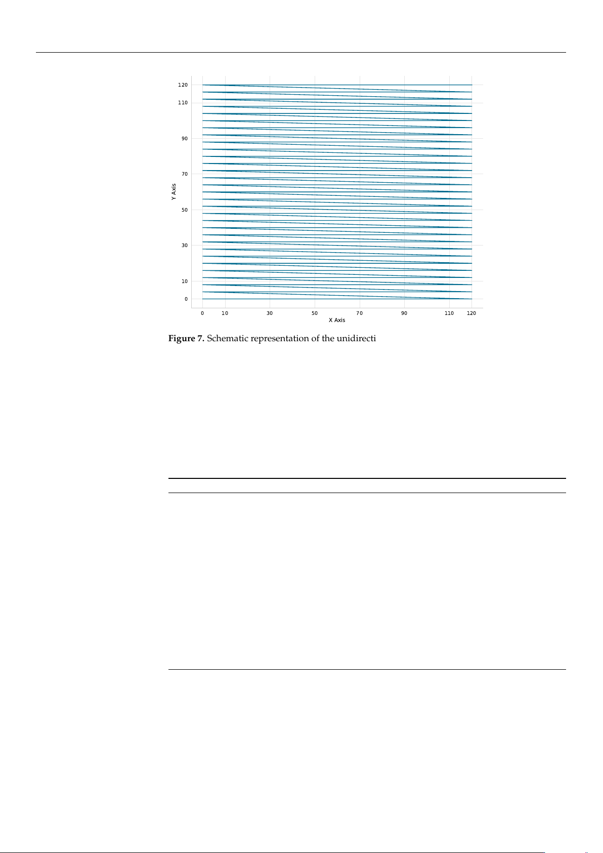
Figure 7. Schematic representation of the unidirectional (left-to-right) scanning strategy employed
by the Reference Coarse algorithm to mitigate backlash and mechanical inconsistencies during
grid exploration.
• Reference Coarse + Fine Scan (Ref-Coarse+Fine):
The Ref-Coarse+Fine scan utilizes a two-stage raster scan process. It begins with a
coarse 6V-step scan (
∼
0.75
µ
m) which is followed by a fine 1V-step scan (
∼
0.125
µ
m) in
a
±
6 V (
±
0.75
µ
m) neighborhood around the coarse maximum. This method provides
the highest accuracy at the cost of increased measurement points. The procedure is
summarized in Algorithm 2.
Algorithm 2 Ref-Coarse+Fine
1: Execute Algorithm 1 (with 6V step) to find (x
coarse
, y
coarse
)
2: P
max
← 0, (x
max
, y
max
) ← (x
coarse
, y
coarse
)
3: for ∆V
x
= −6 to +6 step 1 do
4: for ∆V
y
= −6 to +6 step 1 do
5: V
x
← x
coarse
+ ∆V
x
6: V
y
← y
coarse
+ ∆V
y
7: Move to (V
x
, V
y
) (if within bounds)
8: P ← Measure power
9: if P > P
max
then
10: P
max
← P, (x
max
, y
max
) ← (V
x
, V
y
)
11: end if
12: end for
13: end for
14: Move to (x
max
, y
max
)
• Cross Scan (Cross):
The cross scan method is a two-stage dimensional reduction approach. The algorithm
first performs a coarse cross-scan (4 V steps,
∼
0.5
µ
m) along the X-axis at Y = 60 V
(midrange), and then along the Y-axis at the optimal X position. It then refines the
alignment with fine scans (1 V steps,
∼
0.125
µ
m) in a
±
4 V (
±
0.5
µ
m) neighborhood
around the identified peak. This approach is highly efficient but remains sensitive to
the specific landscape shape. Algorithm 3 outlines this two-stage process.
https://doi.org/10.3390/mi17050592

Micromachines 2026, 17, 592
18 of 34
Algorithm 3 Cross (Two-Stage)
1: // Coarse Stage
2: for V
x
= 0 to 120 step 4 do
3: Sample power at (V
x
, 60)
4: end for
5: Find x
max
with highest power
6: for V
y
= 0 to 120 step 4 do
7: Sample power at (x
max
, V
y
)
8: end for
9: Find y
max
with highest power
10: // Fine Refinement Stage
11: for V
x
= x
max
−4 to x
max
+ 4 step 1 do
12: Sample power at (V
x
, y
max
)
13: end for
14: Find x
f ine
with highest power
15: for V
y
= y
max
−4 to y
max
+ 4 step 1 do
16: Sample power at (x
f ine
, V
y
)
17: end for
18: Move to observed maximum
• Local Bayesian Optimization (Local BO):
The Local BO algorithm first performs a cross-scan to identify the region of interest,
and then applies BO using a GP surrogate model in that local neighborhood (
±
20 V
or
±
2.5
µ
m). This hybrid approach combines the efficiency of initial cross-scan
guidance with the intelligent exploration-exploitation balance of Bayesian methods.
The complete routine is described in Algorithm 4.
Algorithm 4 (Local BO)
1: // Initial cross-scan (7 points per axis)
2: for V
x
∈ {0, 20, 40, 60, 80, 100, 120} do
3: Sample power at (V
x
, 60)
4: end for
5: Find x
max
with highest power
6: for V
y
∈ {0, 20, 40, 60, 80, 100, 120}\{60} do
7: Sample power at (x
max
, V
y
)
8: end for
9: (x
init
, y
init
) ← best point from cross-scan (13 total points)
10: Define search space: x ∈ [x
init
−20, x
init
+ 20], y ∈ [y
init
−20, y
init
+ 20]
11: Sample additional random points to reach 10 initial points in local region
12: Fit Gaussian Process to observations
13: for iteration = 1 to 100 or until convergence do
14: Select next point via Expected Improvement
15: Measure power at selected point
16: Update Gaussian Process
17: if no improvement for 8 iterations then
18: Break
19: end if
20: end for
21: Move to observed maximum
The Expected Improvement (EI) acquisition function balances exploration and
exploitation:
EI(x) = E[max(P(x) − P
max
, 0)] (4)
where P
max
is the current best observed power.
• Global Bayesian Optimization (Global BO):
The Global BO method searches the entire 120 V
×
120 V space (15
µ
m
×
15
µ
m) di-
rectly, without an initial cross-scan phase. This strategy provides the best exploration-
exploitation balance for unknown landscapes through purely probabilistic sampling.
Algorithm 5 details this approach.
https://doi.org/10.3390/mi17050592

Micromachines 2026, 17, 592
19 of 34
Algorithm 5 Global BO
1: Define search space: x ∈ [0, 120], y ∈ [0, 120]
2: Sample 8 Latin-Hypercube sampled points
3: Fit Gaussian Process to observations
4: for iteration = 1 to 70 or until convergence do
5: Select next point via Expected Improvement
6: Measure power at selected point
7: Update Gaussian Process
8: if no improvement for 6 iterations then
9: Break
10: end if
11: end for
12: Move to observed maximum
• Variable Gradient Ascent (Var-Grad):
Var-Grad utilizes an adaptive gradient search logic to maximize alignment speed. The
process begins with a cross-scan initialization (7 points per axis) to identify the initial
signal vicinity, followed by iterative hill-climbing using finite-difference gradient
estimates with a step size of h = 2 V (∼0.25 µm).
The efficiency of this method is driven by an adaptive learning rate (
α
) that scales
inversely with the measured power (P), governed by a gain factor k = 250:
α =
k
max(P, 10
−12
)
(5)
This mechanism allows the algorithm to take aggressive steps in low-power regions
and gradually reduce the step size as it approaches the peak, enabling high-precision
coupling that exploits the system 1 nm hardware resolution. While this approach
achieved the fastest alignment time of 1.18 a.u. in HS-NH simulations, its dependency
on local gradients makes it more susceptible to entrapment in local maxima compared
to probabilistic methods. The pseudo-code for this adaptive approach is provided in
Algorithm 6.
Algorithm 6 Var-Grad
1: // Initial cross-scan (7 points per axis)
2: for V
x
∈ {0, 20, 40, 60, 80, 100, 120} do
3: Sample power at (V
x
, 60)
4: end for
5: Find x
max
with highest power
6: for V
y
∈ {0, 20, 40, 60, 80, 100, 120} \ {60} do
7: Sample power at (x
max
, V
y
)
8: end for
9: (x
0
, y
0
) ← best point from cross-scan
10: Measure P
0
at (x
0
, y
0
)
11: α ← 250/ max(P
0
, 10
−12
) (adaptive learning rate)
12: h ← 2 (finite difference step)
13: for iteration = 1 to 10 do
14: Measure P
1
at (x + h, y), P
2
at (x −h, y)
15: Measure P
3
at (x, y + h), P
4
at (x, y −h)
16: ∇
x
← (P
1
− P
2
)/(2h)
17: ∇
y
← (P
3
− P
4
)/(2h)
18: ∆x ← α ∇
x
, ∆y ← α∇
y
19: x ← x + ∆x, y ← y + ∆ y
20: if |∆x| < 0.5 and |∆y| < 0.5 then
21: Break (convergence)
22: end if
23: end for
24: Move to best observed position
https://doi.org/10.3390/mi17050592