mi17050592.pdf - 第22页

Micromachines 2026 , 17 , 592 22 of 34 T o rigorously account for this non-normal distribution of convergence steps, particu- larly as the number of test scenarios increases, we employ data proﬁles [ 40 ]. A data proﬁle …

Micromachines 2026, 17, 592

21 of 34

(e) Global BO (f) Var-Grad

(g) Fix-Grad

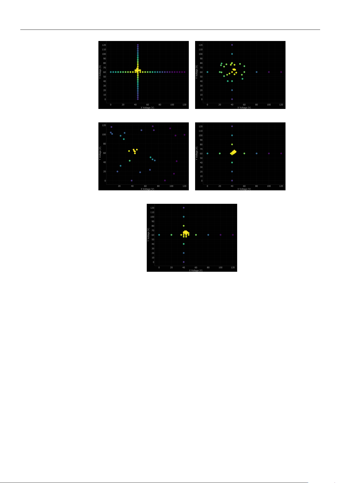
Figure 8. Comparison of all seven alignment algorithms on the same mock scan scenario. Each

panel shows the search path of the algorithm overlaid as discrete colored measurement points,

where the color intensity represents the measured optical power (ranging from dark purple for low

power to bright yellow for the highest power). The ﬁgures demonstrate distinct search strategies:

(a,b) exhaustive raster scanning, (c) dimensional reduction, (d,e) BO with intelligent sampling,

(f,g) gradient-based hill climbing.

3.5. Performance Metrics and Statistical Analysis

Following best practices for algorithm comparison [

], we employ multiple evalua-

tion approaches to ensure a robust assessment. First, for each algorithm on each problem

instance, we record four individual metrics: a binary success indicator (deﬁned as converg-

ing to

≥

95% of the global maximum), the total number of measurement steps required,

the total elapsed time including all movements and settling delays, and the ﬁnal coupling

accuracy (the achieved power divided by the global maximum power).

For the initial performance assessment, we compute a core set of aggregate quantitative

indicators. The primary metric is the overall success rate, strictly deﬁned as the percentage

of alignment problems that were resolved successfully. Furthermore, we calculate central

tendency metrics across all trials—speciﬁcally the mean number of alignment steps, total

execution time, and ﬁnal coupling accuracy. It should be noted that when reporting these

average values, appropriate statistical caveats must be applied to account for the frequently

non-normal distributions inherent in optimization data.

https://doi.org/10.3390/mi17050592

Micromachines 2026, 17, 592

22 of 34

To rigorously account for this non-normal distribution of convergence steps, particu-

larly as the number of test scenarios increases, we employ data proﬁles [

]. A data proﬁle

plots the fraction of problems solved as a function of the number of function evaluations

(measurement steps):

(k) =

|P|

|{p ∈ P : n

s,p

≤ k}| (6)

where

is the set of test problems,

is a solver (algorithm),

s,p

is the number of steps

required by solver

on problem

, and

is the step budget. Data proﬁles provide a

complete picture of algorithm performance by showing not just average behavior, but the

full distribution of convergence speeds. An algorithm with a steep data proﬁle quickly

solves most problems, while a shallow proﬁle indicates slower or less reliable convergence.

In this work, data proﬁles are generated for the experimental results and for each speciﬁc

simulation scenario (HS-H, HS-NH, LS-H, and LS-NH), enabling a comprehensive statistical

comparison of algorithm performance across all operating conditions.

4. Results

4.1. Experimental Results

The algorithms are ranked based on a composite evaluation considering four critical

metrics: (1) success rate, which is the primary criterion for production deployment; (2) av-

erage alignment time, reﬂecting throughput impact; (3) ﬁnal accuracy, indicating optical

coupling quality; and (4) average number of steps, representing measurement efﬁciency.

Algorithms with 100% success rate are prioritized, then ranked by alignment time. Those

with lower success rates are ranked lower regardless of speed, as unreliable alignment

requires manual intervention and severely impacts production throughput.

Table 1 summarizes the performance of all seven algorithms across the eight experi-

mental coupling scenarios.

Table 1. Experimental alignment results across 8 coupling scenarios. Algorithms ranked by combined

performance considering success rate, time, accuracy, and measurement efﬁciency. Results obtained

with baseline algorithm parameters.

Rank Method Success Rate Avg Time (a.u.) Avg Accuracy (%) Avg Steps

1 Local BO 100% 99.87 98.24 26.5

2 Fix-Grad 100% 154.01 99.18 69.0

3 Global BO 87.5% 175.19 97.60 37.4

4 Ref-Coarse+Fine 87.5% 334.11 98.31 600.3

5 Cross 75.0% 36.63 96.84 80.0

6 Var-Grad 75.0% 59.28 95.99 22.5

7 Ref-Coarse 75.0% 410.90 96.81 961.0

Experimental results indicate that the Local BO method achieves superior overall

performance, delivering a 100% success rate, 98.24% accuracy, and rapid convergence

(26.5 steps, 99.87 a.u.). This hybrid approach successfully balances exploration and ex-

ploitation via cross-scan initialization followed by Bayesian reﬁnement. The Fix-Grad

algorithm similarly achieves absolute reliability (100% success) alongside a marginally

higher accuracy of 99.18%, although its systematic neighborhood exploration demands

increased execution metrics (69.0 steps, 154.01 a.u.). In contrast, Global BO demonstrates

strong general performance (97.60% accuracy, 37.4 steps) but yields an 87.5% success rate,

indicating occasional difﬁculty navigating complex landscapes where optimal coupling re-

gions remain distant from initial random samples. Furthermore, while the Ref-Coarse+Fine

strategy provides adequate accuracy (98.31%), the exhaustive measurement requirement

https://doi.org/10.3390/mi17050592

Micromachines 2026, 17, 592

23 of 34

(600.3 steps, 334.11 a.u.) renders the approach entirely impractical for high-throughput

manufacturing. The remaining techniques, that are Cross, Var-Grad, and Reference Coarse,

exhibit heightened sensitivity to landscape topology, peaking at a 75% success rate. No-

tably, Var-Grad operates with the highest speed (22.5 steps, 59.28 a.u.) but lacks requisite

dependability. Consequently, Local BO presents the optimal synthesis of speed, accuracy,

and reliability for physical alignment tasks. Securing a 100% success rate is paramount

for strict production environments to eliminate manual intervention and preserve critical

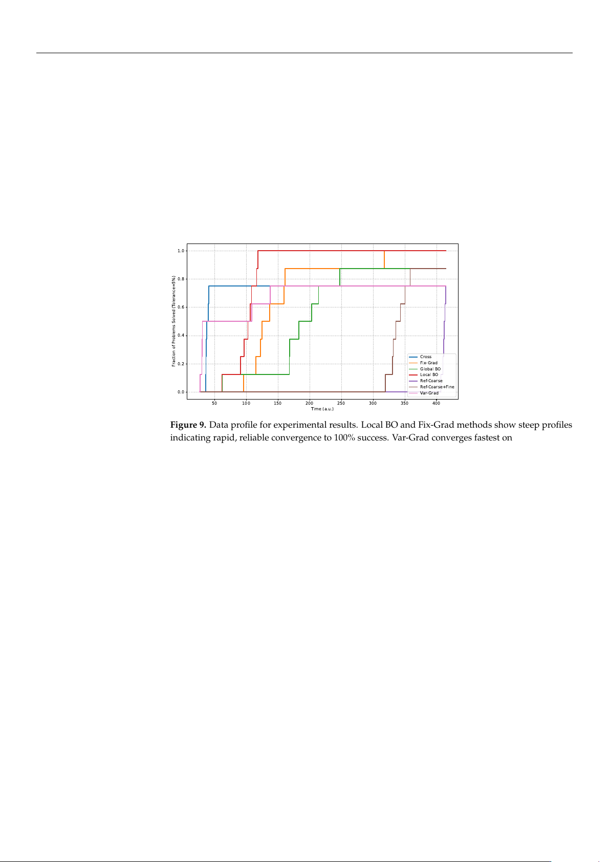
operational throughput. Figure 9 shows the data proﬁle for experimental results, plotting

the fraction of problems solved as a function of total alignment time. The discrete, step-like

appearance of these proﬁles is simply a consequence of the limited experimental sample

size (N = 8).

50 100 150 200 250 300 350 400

Time (a.u.)

0.0

0.2

0.4

0.6

0.8

1.0

Fraction of Problems Solved (Tolerance=5%)

Cross

Fix-Grad

Global BO

Local BO

Ref-Coarse

Ref-Coarse+Fine

Var-Grad

Figure 9. Data proﬁle for experimental results. Local BO and Fix-Grad methods show steep proﬁles

indicating rapid, reliable convergence to 100% success. Var-Grad converges fastest on easy problems

but plateaus at 75%, while Ref-Coarse/Ref-Coarse+Fine require many measurements.

Following the methodology of Beiranvand et al. [

], data proﬁle analysis elucidates

comprehensive convergence behaviors that simple central tendency metrics obscure. Specif-

ically, the Local BO proﬁle exhibits a steep initial trajectory, achieving 100% success rate

within approximately 30 steps. The Fix-Grad method similarly reaches absolute reliability

by 80 steps, demonstrating a steady, albeit slower, progression. Conversely, algorithms

such as Global BO, Var-Grad, and Cross exhibit rapid initial climbs but prematurely plateau

at success rates of 87.5%, 75%, and 75%, respectively, indicating fundamental failure cases.

Moreover, the exhaustive reference techniques Ref-Coarse and Ref-Coarse+Fine require

hundreds of measurements merely to attain sub-optimal success rates between 75% and

87.5%. Ultimately, this statistical visualization demonstrates that while Var-Grad yields

the lowest average step count (22.5), its early performance plateau and 25% failure rate

render it signiﬁcantly inferior to the robust Local BO and Fix-Grad algorithms for rigorous

production deployment.

4.2. Simulation Results

Table 2 summarizes the average number of measurement steps required by each

algorithm across the four simulation scenarios. Results are averaged over multiple mock

ﬁles generated from the experimental data. Global BO requires the fewest steps (

∼

25),

followed closely by Var-Grad (

∼

26) and Local BO (

∼

31). The intelligent sampling of

Bayesian and Gradient methods reduces the measurement burden by over 20

compared

to Ref-Coarse+Fine scanning (540 steps). The step counts are independent of the operating

scenario, as they reﬂect algorithmic logic rather than timing. However, these step counts

directly impact total time, which varies signiﬁcantly across scenarios as shown next.

https://doi.org/10.3390/mi17050592