mi17050592.pdf - 第20页
Micromachines 2026 , 17 , 592 20 of 34 • Fixed Gradient Ascent (Fix-Grad): The Fix-Grad method is a traditional gradient sear ch technique with fixed step sizes that halve upon observing no improvement. The procedure begi…

Micromachines 2026, 17, 592
19 of 34
Algorithm 5 Global BO
1: Define search space: x ∈ [0, 120], y ∈ [0, 120]
2: Sample 8 Latin-Hypercube sampled points
3: Fit Gaussian Process to observations
4: for iteration = 1 to 70 or until convergence do
5: Select next point via Expected Improvement
6: Measure power at selected point
7: Update Gaussian Process
8: if no improvement for 6 iterations then
9: Break
10: end if
11: end for
12: Move to observed maximum
• Variable Gradient Ascent (Var-Grad):
Var-Grad utilizes an adaptive gradient search logic to maximize alignment speed. The
process begins with a cross-scan initialization (7 points per axis) to identify the initial
signal vicinity, followed by iterative hill-climbing using finite-difference gradient
estimates with a step size of h = 2 V (∼0.25 µm).
The efficiency of this method is driven by an adaptive learning rate (
α
) that scales
inversely with the measured power (P), governed by a gain factor k = 250:
α =
k
max(P, 10
−12
)
(5)
This mechanism allows the algorithm to take aggressive steps in low-power regions
and gradually reduce the step size as it approaches the peak, enabling high-precision
coupling that exploits the system 1 nm hardware resolution. While this approach
achieved the fastest alignment time of 1.18 a.u. in HS-NH simulations, its dependency
on local gradients makes it more susceptible to entrapment in local maxima compared
to probabilistic methods. The pseudo-code for this adaptive approach is provided in
Algorithm 6.
Algorithm 6 Var-Grad
1: // Initial cross-scan (7 points per axis)
2: for V
x
∈ {0, 20, 40, 60, 80, 100, 120} do
3: Sample power at (V
x
, 60)
4: end for
5: Find x
max
with highest power
6: for V
y
∈ {0, 20, 40, 60, 80, 100, 120} \ {60} do
7: Sample power at (x
max
, V
y
)
8: end for
9: (x
0
, y
0
) ← best point from cross-scan
10: Measure P
0
at (x
0
, y
0
)
11: α ← 250/ max(P
0
, 10
−12
) (adaptive learning rate)
12: h ← 2 (finite difference step)
13: for iteration = 1 to 10 do
14: Measure P
1
at (x + h, y), P
2
at (x −h, y)
15: Measure P
3
at (x, y + h), P
4
at (x, y −h)
16: ∇
x
← (P
1
− P
2
)/(2h)
17: ∇
y
← (P
3
− P
4
)/(2h)
18: ∆x ← α ∇
x
, ∆y ← α∇
y
19: x ← x + ∆x, y ← y + ∆ y
20: if |∆x| < 0.5 and |∆y| < 0.5 then
21: Break (convergence)
22: end if
23: end for
24: Move to best observed position
https://doi.org/10.3390/mi17050592
Micromachines 2026, 17, 592
20 of 34
• Fixed Gradient Ascent (Fix-Grad):
The Fix-Grad method is a traditional gradient search technique with fixed step sizes
that halve upon observing no improvement. The procedure begins with a cross-scan
(7 points per axis), and then iteratively explores neighbors in the cardinal directions
(initial step 4 V or
∼
0.5
µ
m, minimum 1 V or
∼
0.125
µ
m) to identify the optimal ascent
direction, as shown in Algorithm 7:
Algorithm 7 Fix-Grad
1: // Initial cross-scan (7 points per axis)
2: for V
x
∈ {0, 20, 40, 60, 80, 100, 120} do
3: Sample power at (V
x
, 60)
4: end for
5: Find x
max
with highest power
6: for V
y
∈ {0, 20, 40, 60, 80, 100, 120}\ {60} do
7: Sample power at (x
max
, V
y
)
8: end for
9: (x
0
, y
0
) ← best point from cross-scan
10: Measure P
current
at (x
0
, y
0
)
11: δ ← 4 (initial step size)
12: while δ ≥ 1 do
13: Measure power at (x + δ, y), (x −δ, y), (x, y + δ), (x, y −δ)
14: (x
′
, y
′
, P
′
) ← best neighbor
15: if P
′
> P
current
then
16: (x, y, P
current
) ← (x
′
, y
′
, P
′
)
17: else
18: δ ← δ/2 (reduce step size)
19: end if
20: end while
21: Move to (x, y)
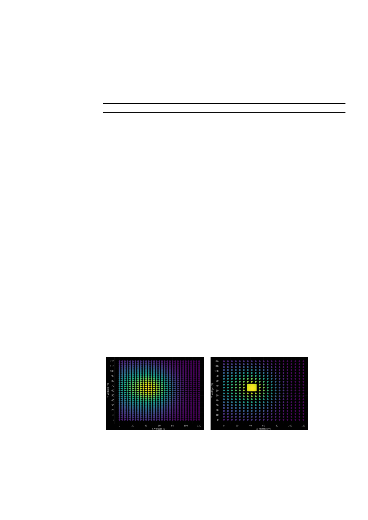
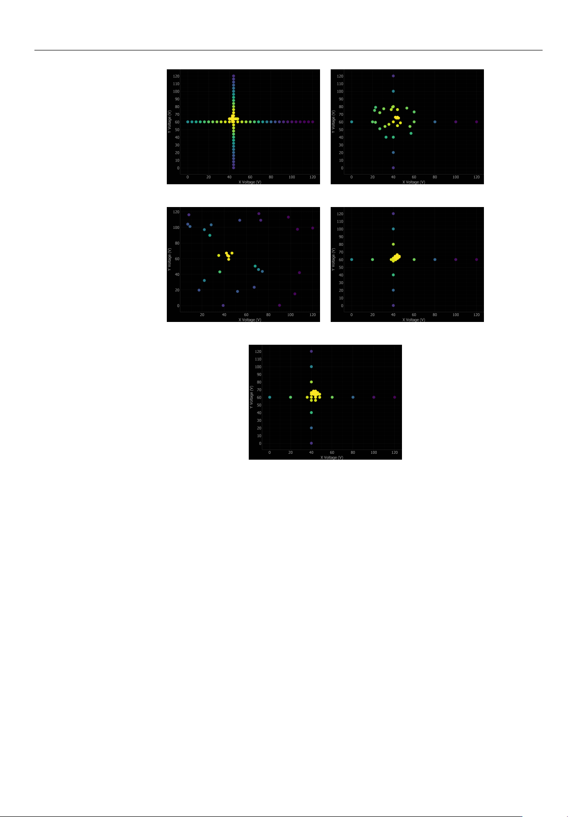
Figure 8 illustrates the application of all seven alignment algorithms to a representative
mock scan scenario centered at (60 V, 60 V), providing a direct visual comparison of
their respective search strategies. Each algorithm navigates the 120 V
×
120 V operating
range using a distinct optimization philosophy: Ref-Coarse and Ref-Coarse+Fine employ
systematic raster scans; Cross scan utilizes dimensional reduction via orthogonal axis
scanning; Local and Global BO implement intelligent sampling guided by Gaussian Process
uncertainty; and Variable and Fix-Grad utilize hill-climbing techniques to track the local
power gradient.
(a) Ref-Coarse (b) Ref-Coarse+Fine
Figure 8. Cont.
https://doi.org/10.3390/mi17050592
Micromachines 2026, 17, 592
21 of 34
(c) Cross (d) Local BO
(e) Global BO (f) Var-Grad
(g) Fix-Grad
Figure 8. Comparison of all seven alignment algorithms on the same mock scan scenario. Each
panel shows the search path of the algorithm overlaid as discrete colored measurement points,
where the color intensity represents the measured optical power (ranging from dark purple for low
power to bright yellow for the highest power). The figures demonstrate distinct search strategies:
(a,b) exhaustive raster scanning, (c) dimensional reduction, (d,e) BO with intelligent sampling,
(f,g) gradient-based hill climbing.
3.5. Performance Metrics and Statistical Analysis
Following best practices for algorithm comparison [
18
], we employ multiple evalua-
tion approaches to ensure a robust assessment. First, for each algorithm on each problem
instance, we record four individual metrics: a binary success indicator (defined as converg-
ing to
≥
95% of the global maximum), the total number of measurement steps required,
the total elapsed time including all movements and settling delays, and the final coupling
accuracy (the achieved power divided by the global maximum power).
For the initial performance assessment, we compute a core set of aggregate quantitative
indicators. The primary metric is the overall success rate, strictly defined as the percentage
of alignment problems that were resolved successfully. Furthermore, we calculate central
tendency metrics across all trials—specifically the mean number of alignment steps, total
execution time, and final coupling accuracy. It should be noted that when reporting these
average values, appropriate statistical caveats must be applied to account for the frequently
non-normal distributions inherent in optimization data.
https://doi.org/10.3390/mi17050592