mi17050592.pdf - 第16页
Micromachines 2026 , 17 , 592 16 of 34 ward (incr easing voltage) path. This approach avoids the unpr edictable displacement that would occur if the system attempted to follow the r eturn (decr easing voltage) hyster esi…

Micromachines 2026, 17, 592
15 of 34
3.3.3. Algorithm Verification
A Headless Aligner script replicates the logic of the main controller. It loads each
of the 9 mock files as a virtual device (simulating slew rates and settling times) and
runs all 7 alignment strategies sequentially. For every single one of the 9 mock files,
the simulation generates 7 result files, one for each algorithm, totaling 63 result files per
experimental dataset.
Each generated result file provides a comprehensive record of the alignment procedure.
Specifically, it includes a detailed path log that tracks every X and Y coordinate step
executed by the algorithm, alongside the corresponding simulated optical power measured
at each discrete position. Furthermore, the file incorporates a concluding summary that
details the total number of measurement points, the final maximum optical power achieved,
and the total execution time. This total alignment time is rigorously calculated by factoring
in a simulated hardware slew rate of 100 V/s combined with a constant mechanical settling
buffer. To ensure the comparison focuses strictly on algorithmic efficiency rather than
hardware-specific speeds, all alignment times throughout this work are expressed in
arbitrary units (a.u.). For this normalization, the baseline execution time of the Local BO
method under the original LS-H configuration is defined as exactly 100.0 a.u. By comparing
these files across all mock scenarios, we can quantify which algorithm is the fastest and
most accurate for diverse device profiles.
3.3.4. Hardware Simulation
The simulated hardware model is designed to accurately mimic the mechanical and
electrical behavior of the physical alignment system across several key operational pa-
rameters. As already discussed, to realistically capture movement timing, the model
incorporates two distinct regimes: a HS (high-speed) operation characterized by a rapid
slew rate and abbreviated settling times, and a LS (low-speed) operation that employs
a more conservative slew rate alongside extended settling durations. Furthermore, the
model strictly enforces physical position limits, constraining the simulated actuator travel
to a bounded 0–15
µ
m range (corresponding to a 0–120 V drive signal) across both the X
and Y axes. Finally, to simulate dynamic feedback, optical power measurements at any
given coordinate are continuously evaluated via direct interpolation from the previously
constructed RBF surface, ensuring realistic continuous domain responses during the virtual
alignment process.
For hysteresis modeling, when the target position is lower than the current position in
either axis, the system simulates a reset-to-zero followed by a move-to-target, approximat-
ing the piezoelectric hysteresis behavior according to:
t
move
=
d
reset
v
+
d
target
v
+ 2t
settle
if x
target
< x
current
or y
target
< y
current
d
direct
v
+ t
settle
otherwise
(2)
where the voltage distance terms are defined as:
d
reset
=
q
x
2
current
+ y
2
current
d
target
=
q
x
2
target
+ y
2
target
d
direct
=
q
(x
target
− x
current
)
2
+ (y
target
−y
current
)
2
(3)
with v representing the effective slew rate and t
settle
the settling time.
This reset-to-zero strategy ensures that when moving to a lower voltage position, the
system first returns to the origin (0, 0) and then moves to the target position along the for-
https://doi.org/10.3390/mi17050592

Micromachines 2026, 17, 592
16 of 34
ward (increasing voltage) path. This approach avoids the unpredictable displacement that
would occur if the system attempted to follow the return (decreasing voltage) hysteresis
path, thereby ensuring repeatable positioning at the cost of additional movement time. To
evaluate the absolute worst-case temporal penalty of open-loop hysteresis, the simulation
utilizes this simplified reset-to-zero mathematical model. While advanced analytical feed-
forward models exist, forcing a physical return to the origin for every negative voltage step
allows us to reliably benchmark the maximum timing overhead an algorithm might incur
in the absence of complex software compensation.
3.4. Alignment Algorithms
We evaluate seven alignment algorithms deliberately selected to represent the com-
plete methodological spectrum of optical optimization strategies. These seven methods
span four distinct paradigms: (1) exhaustive grid searches (Reference Coarse, Reference
Coarse+Fine) that establish fundamental ground-truth baselines; (2) dimensional reduction
techniques (Cross Scan) that represent standard industry heuristics; (3) deterministic hill-
climbing approaches (Fixed and Variable Gradient Ascent) that prioritize rapid, localized
convergence; and (4) probabilistic machine-learning models (Local and Global Bayesian
Optimization) designed to navigate noisy, hysteresis-distorted landscapes. By compar-
ing this specific set, we can systematically evaluate the fundamental trade-offs between
measurement efficiency, computational overhead, and ultimate alignment reliability. The
algorithm descriptions below reflect the refined parameters and logic utilized during the
simulation study. Specifically, the operational mechanics for each of the seven evaluated
methods are detailed as follows:
• Reference Coarse Scan (Ref-Coarse):
The reference coarse scan consists of an exhaustive raster scan with 4V voltage steps
(corresponding to
∼
0.5
µ
m spatial steps), followed by a move to the maximum de-
tected power position. This establishes a baseline for global search, as detailed in
Algorithm 1.
Algorithm 1 Ref-Coarse
1: P
max
← 0, (x
max
, y
max
) ← (0, 0)
2: for V
x
= 0 to 120 step 4 do
3: for V
y
= 0 to 120 step 4 do
4: Move to (V
x
, V
y
)
5: P ← Measure power
6: if P > P
max
then
7: P
max
← P, (x
max
, y
max
) ← (V
x
, V
y
)
8: end if
9: end for
10: end for
11: Move to (x
max
, y
max
)
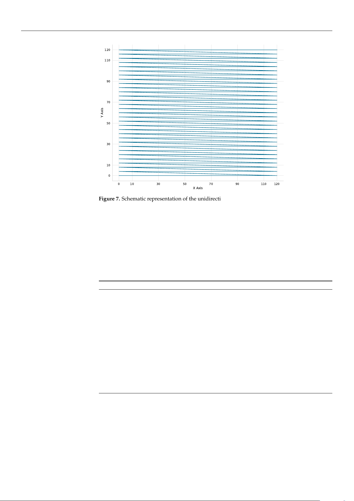
As illustrated in Figure 7, the Reference Coarse scan employs a strictly unidirec-
tional (left-to-right) scanning strategy. This pattern is specifically designed to mit-
igate mechanical backlash and hysteresis inconsistencies during the exhaustive
grid exploration.
https://doi.org/10.3390/mi17050592
Micromachines 2026, 17, 592
17 of 34
0 10 30 50 70 90 110 120
X Axis
0
10
30
50
70
90
110
120
Y Axis
Figure 7. Schematic representation of the unidirectional (left-to-right) scanning strategy employed
by the Reference Coarse algorithm to mitigate backlash and mechanical inconsistencies during
grid exploration.
• Reference Coarse + Fine Scan (Ref-Coarse+Fine):
The Ref-Coarse+Fine scan utilizes a two-stage raster scan process. It begins with a
coarse 6V-step scan (
∼
0.75
µ
m) which is followed by a fine 1V-step scan (
∼
0.125
µ
m) in
a
±
6 V (
±
0.75
µ
m) neighborhood around the coarse maximum. This method provides
the highest accuracy at the cost of increased measurement points. The procedure is
summarized in Algorithm 2.
Algorithm 2 Ref-Coarse+Fine
1: Execute Algorithm 1 (with 6V step) to find (x
coarse
, y
coarse
)
2: P
max
← 0, (x
max
, y
max
) ← (x
coarse
, y
coarse
)
3: for ∆V
x
= −6 to +6 step 1 do
4: for ∆V
y
= −6 to +6 step 1 do
5: V
x
← x
coarse
+ ∆V
x
6: V
y
← y
coarse
+ ∆V
y
7: Move to (V
x
, V
y
) (if within bounds)
8: P ← Measure power
9: if P > P
max
then
10: P
max
← P, (x
max
, y
max
) ← (V
x
, V
y
)
11: end if
12: end for
13: end for
14: Move to (x
max
, y
max
)
• Cross Scan (Cross):
The cross scan method is a two-stage dimensional reduction approach. The algorithm
first performs a coarse cross-scan (4 V steps,
∼
0.5
µ
m) along the X-axis at Y = 60 V
(midrange), and then along the Y-axis at the optimal X position. It then refines the
alignment with fine scans (1 V steps,
∼
0.125
µ
m) in a
±
4 V (
±
0.5
µ
m) neighborhood
around the identified peak. This approach is highly efficient but remains sensitive to
the specific landscape shape. Algorithm 3 outlines this two-stage process.
https://doi.org/10.3390/mi17050592