mi17050592.pdf - 第14页
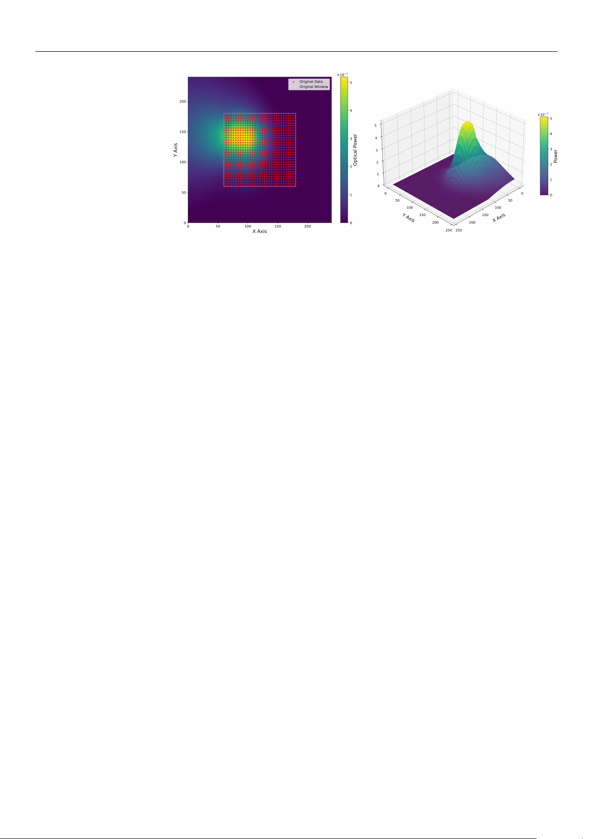
Micromachines 2026 , 17 , 592 14 of 34 ( a ) ( b ) Figure 6. Reconstructed optical power surface from experimental data. ( a ) 2D heatmap showing the 240 × 240 global grid with centered experimental data points (red mark…
Micromachines 2026, 17, 592
13 of 34
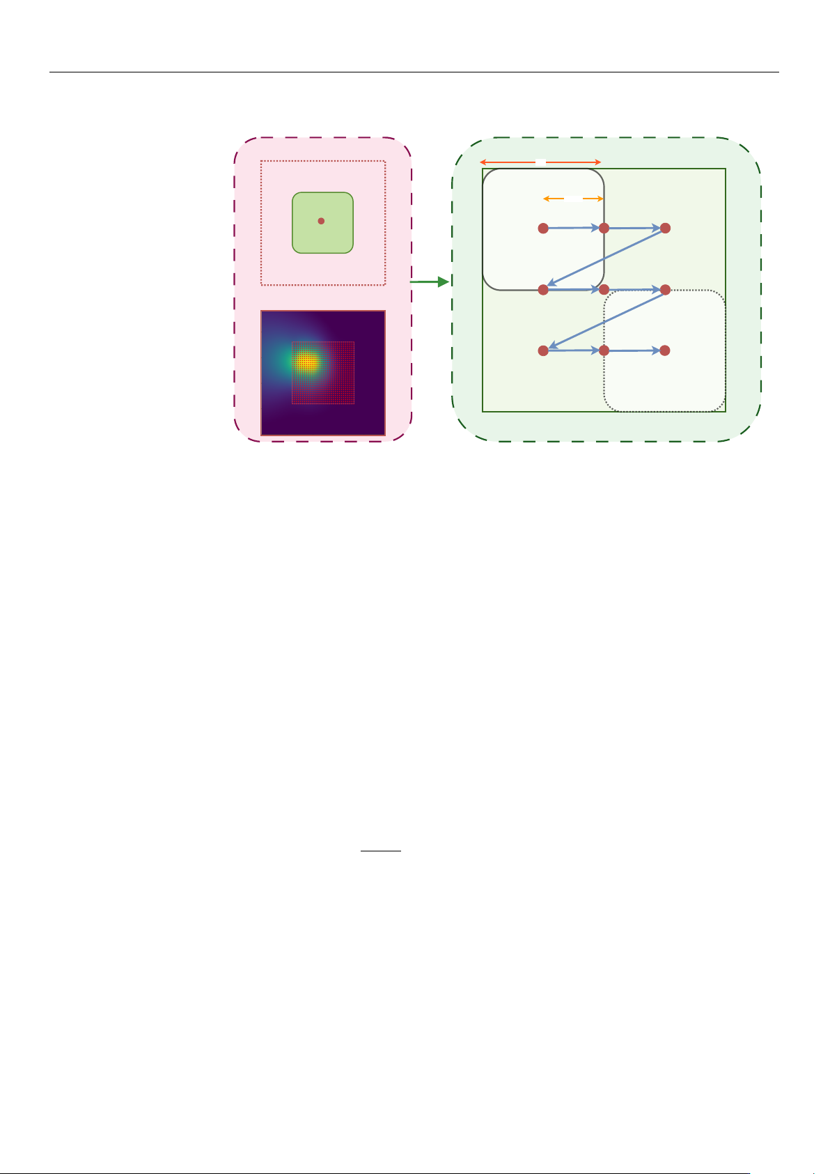
The framework has three main components, as described in the following.
STEP 2: RBF Fitting → Ground Truth
(240×240)
STEP 3: Sliding Window Extraction (120×120 windows, 60 step)
0,0
240,0
0,240
240,240
1
9
120
60 step
STEP 1: Input Data + Centering
Input 120×120
data Centered
(120, 120)
Figure 5. Simulation workflow used to generate synthetic alignment scenarios from experimental
scans and to evaluate alignment algorithms under different operating regimes. Experimental data are
reconstructed into a high-resolution coupling surface, windowed into multiple mock scenarios, and
then replayed through the hardware timing model (with/without reset-to-zero hysteresis strategy) to
produce comparable metrics across the four scenarios.
3.3.1. Surface Reconstruction and Centering
Starting from experimental scan data, we use RBF interpolation with multiquadric ker-
nel to create smooth coupling surfaces. The process consists of the following critical steps.
1.
Centering Strategy: The simulation standardizes the input data before fitting. It
computes the geometric center of the raw input scan and shifts the data so that it
aligns with the center (120, 120) of the global simulation grid. This ensures that the
peak is always accessible and not cut off at the edges of the simulation environment.
2.
Normalization: To ensure numerical stability during interpolation, the coordinates
are temporarily normalized to a 0–1 range.
3.
RBF Fitting: We utilize SciPy RBF interpolation function [
43
] with a multiquadric
kernel and smoothing factor (ϵ = 0.01) to create a mathematical surface:
P(x, y) =
N
∑
i=1
w
i
ϕ(∥[x, y] − [x
i
, y
i
]∥) (1)
where
ϕ(r) =
√
r
2
+ ϵ
2
is the multiquadric basis function,
w
i
are interpolation weights
determined from experimental data points (x
i
, y
i
, P
i
), and ϵ is the smoothing parameter.
4.
Grid Generation: A dense 240
×
240 pixel grid is generated, representing the ground-
truth power values for every possible coordinate in the simulation area. This creates a
continuous surface from the discrete experimental measurements.
Figure 6 illustrates this surface reconstruction process. The heatmap (a) shows the
interpolated power landscape on the 240
×
240 global grid, with the original experimental
data points (red markers) centered at (120, 120) and the dashed rectangle indicating the orig-
inal 120
×
120 measurement window. The 3D surface plot (b) provides a three-dimensional
visualization of the optical coupling landscape, clearly showing the peak power region and
the smooth interpolation that extends beyond the measured data points.
https://doi.org/10.3390/mi17050592
Micromachines 2026, 17, 592
14 of 34
(a) (b)
Figure 6. Reconstructed optical power surface from experimental data. (a) 2D heatmap showing the
240
×
240 global grid with centered experimental data points (red markers within dashed rectangle).
(b) 3D surface visualization showing the smooth RBF interpolation and peak power region. The
surface extends beyond the measured region to create multiple mock test scenarios.
3.3.2. Environmental Simulation (Mock Scan Generation)
Real alignment hardware has a limited field of view corresponding to the piezoelectric
actuator range (120 V, equivalent to 15
µ
m displacement), while the simulated surface
is 240 units wide. To test algorithm robustness, the large surface is divided into smaller,
realistic views using a systematic sliding window technique, according to the following.
1.
Sliding Window Process: The sliding window process employs a fixed window size
of 120
×
120 units, which corresponds directly to the typical 0–120 V operating
range of the piezoelectric stage. To systematically evaluate the data, this window is
translated across the global 240
×
240 data matrix using a discrete step size of 60 units.
Originating at the (0, 0) coordinate of the global grid, the window slides through
sequential positions, such as (0, 60), (0, 120), and (60, 0), ensuring comprehensive and
overlapping coverage of the entire surface area in a structured grid pattern.
2.
Coordinate Localization: As the window moves to different positions (e.g., Global
X = 60 to 180), the system transforms the extracted data back to local coordinates
(0–120 V) by subtracting the offset from the window origin. This is critical, as it
ensures that the algorithms perceive every file as a standard 0–120 V hardware range,
indistinguishable from real operation.
3.
Mock File Generation: This systematic windowing process generates 9 distinct mock
CSV files from each experimental dataset. Each file contains only the X, Y, and Power
data visible within that specific 120 V
×
120 V window at offsets of 0, 60, and 120 V
in both dimensions. This forces the algorithms to locate the peak in various contexts
(e.g., peak centered, peak at the edge, or low-power regions), providing a rigorous
test of algorithm robustness across diverse initial conditions.
To provide a statistically rigorous benchmark, a comprehensive simulation library was
constructed from the 8 experimental datasets. Each experimental scan was interpolated
onto a 240
×
240 voltage grid using a multiquadric RBF to serve as a ground-truth coupling
landscape. From these, a total of 72 unique test scenarios (8 experiments
×
9 systematic
spatial offsets) were generated by extracting 120 V
×
120 V sub-windows at varying spatial
positions (offsets of 0, 60, and 120 V in each dimension). This systematic procedure ensures
that the algorithms are evaluated against a diverse set of initial peak positions relative to
the scan window, simulating a wide range of initial fiber-to-chip misalignments that might
occur in production testing.
https://doi.org/10.3390/mi17050592

Micromachines 2026, 17, 592
15 of 34
3.3.3. Algorithm Verification
A Headless Aligner script replicates the logic of the main controller. It loads each
of the 9 mock files as a virtual device (simulating slew rates and settling times) and
runs all 7 alignment strategies sequentially. For every single one of the 9 mock files,
the simulation generates 7 result files, one for each algorithm, totaling 63 result files per
experimental dataset.
Each generated result file provides a comprehensive record of the alignment procedure.
Specifically, it includes a detailed path log that tracks every X and Y coordinate step
executed by the algorithm, alongside the corresponding simulated optical power measured
at each discrete position. Furthermore, the file incorporates a concluding summary that
details the total number of measurement points, the final maximum optical power achieved,
and the total execution time. This total alignment time is rigorously calculated by factoring
in a simulated hardware slew rate of 100 V/s combined with a constant mechanical settling
buffer. To ensure the comparison focuses strictly on algorithmic efficiency rather than
hardware-specific speeds, all alignment times throughout this work are expressed in
arbitrary units (a.u.). For this normalization, the baseline execution time of the Local BO
method under the original LS-H configuration is defined as exactly 100.0 a.u. By comparing
these files across all mock scenarios, we can quantify which algorithm is the fastest and
most accurate for diverse device profiles.
3.3.4. Hardware Simulation
The simulated hardware model is designed to accurately mimic the mechanical and
electrical behavior of the physical alignment system across several key operational pa-
rameters. As already discussed, to realistically capture movement timing, the model
incorporates two distinct regimes: a HS (high-speed) operation characterized by a rapid
slew rate and abbreviated settling times, and a LS (low-speed) operation that employs
a more conservative slew rate alongside extended settling durations. Furthermore, the
model strictly enforces physical position limits, constraining the simulated actuator travel
to a bounded 0–15
µ
m range (corresponding to a 0–120 V drive signal) across both the X
and Y axes. Finally, to simulate dynamic feedback, optical power measurements at any
given coordinate are continuously evaluated via direct interpolation from the previously
constructed RBF surface, ensuring realistic continuous domain responses during the virtual
alignment process.
For hysteresis modeling, when the target position is lower than the current position in
either axis, the system simulates a reset-to-zero followed by a move-to-target, approximat-
ing the piezoelectric hysteresis behavior according to:
t
move
=
d
reset
v
+
d
target
v
+ 2t
settle
if x
target
< x
current
or y
target
< y
current
d
direct
v
+ t
settle
otherwise
(2)
where the voltage distance terms are defined as:
d
reset
=
q
x
2
current
+ y
2
current
d
target
=
q
x
2
target
+ y
2
target
d
direct
=
q
(x
target
− x
current
)
2
+ (y
target
−y
current
)
2
(3)
with v representing the effective slew rate and t
settle
the settling time.
This reset-to-zero strategy ensures that when moving to a lower voltage position, the
system first returns to the origin (0, 0) and then moves to the target position along the for-
https://doi.org/10.3390/mi17050592