mi17050592.pdf - 第17页
Micromachines 2026 , 17 , 592 17 of 34 0 10 30 50 70 90 110 120 X Axis 0 10 30 50 70 90 110 120 Y Axis Figure 7. Schematic r epresentation of the unidir ectional (left-to-right) scanning strategy employed by the Referenc…

Micromachines 2026, 17, 592
16 of 34
ward (increasing voltage) path. This approach avoids the unpredictable displacement that
would occur if the system attempted to follow the return (decreasing voltage) hysteresis
path, thereby ensuring repeatable positioning at the cost of additional movement time. To
evaluate the absolute worst-case temporal penalty of open-loop hysteresis, the simulation
utilizes this simplified reset-to-zero mathematical model. While advanced analytical feed-
forward models exist, forcing a physical return to the origin for every negative voltage step
allows us to reliably benchmark the maximum timing overhead an algorithm might incur
in the absence of complex software compensation.
3.4. Alignment Algorithms
We evaluate seven alignment algorithms deliberately selected to represent the com-
plete methodological spectrum of optical optimization strategies. These seven methods
span four distinct paradigms: (1) exhaustive grid searches (Reference Coarse, Reference
Coarse+Fine) that establish fundamental ground-truth baselines; (2) dimensional reduction
techniques (Cross Scan) that represent standard industry heuristics; (3) deterministic hill-
climbing approaches (Fixed and Variable Gradient Ascent) that prioritize rapid, localized
convergence; and (4) probabilistic machine-learning models (Local and Global Bayesian
Optimization) designed to navigate noisy, hysteresis-distorted landscapes. By compar-
ing this specific set, we can systematically evaluate the fundamental trade-offs between
measurement efficiency, computational overhead, and ultimate alignment reliability. The
algorithm descriptions below reflect the refined parameters and logic utilized during the
simulation study. Specifically, the operational mechanics for each of the seven evaluated
methods are detailed as follows:
• Reference Coarse Scan (Ref-Coarse):
The reference coarse scan consists of an exhaustive raster scan with 4V voltage steps
(corresponding to
∼
0.5
µ
m spatial steps), followed by a move to the maximum de-
tected power position. This establishes a baseline for global search, as detailed in
Algorithm 1.
Algorithm 1 Ref-Coarse
1: P
max
← 0, (x
max
, y
max
) ← (0, 0)
2: for V
x
= 0 to 120 step 4 do
3: for V
y
= 0 to 120 step 4 do
4: Move to (V
x
, V
y
)
5: P ← Measure power
6: if P > P
max
then
7: P
max
← P, (x
max
, y
max
) ← (V
x
, V
y
)
8: end if
9: end for
10: end for
11: Move to (x
max
, y
max
)
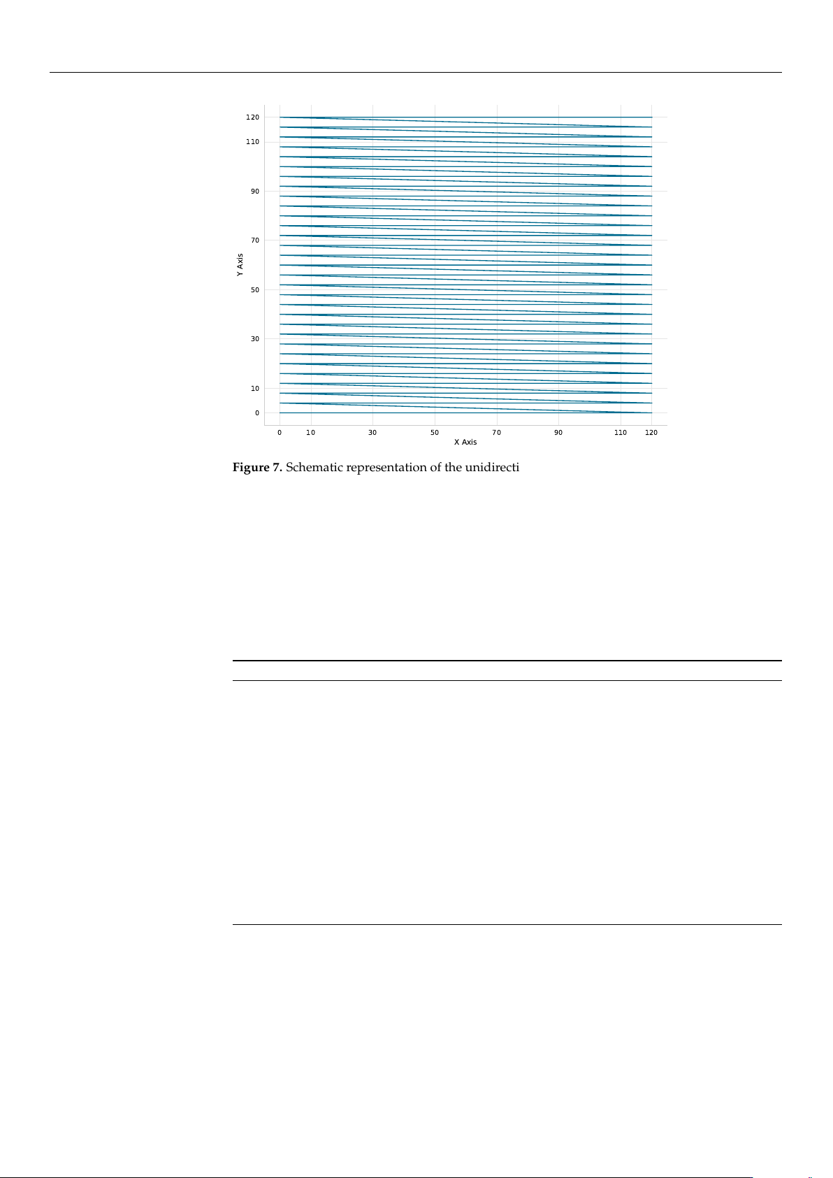
As illustrated in Figure 7, the Reference Coarse scan employs a strictly unidirec-
tional (left-to-right) scanning strategy. This pattern is specifically designed to mit-
igate mechanical backlash and hysteresis inconsistencies during the exhaustive
grid exploration.
https://doi.org/10.3390/mi17050592
Micromachines 2026, 17, 592
17 of 34
0 10 30 50 70 90 110 120
X Axis
0
10
30
50
70
90
110
120
Y Axis
Figure 7. Schematic representation of the unidirectional (left-to-right) scanning strategy employed
by the Reference Coarse algorithm to mitigate backlash and mechanical inconsistencies during
grid exploration.
• Reference Coarse + Fine Scan (Ref-Coarse+Fine):
The Ref-Coarse+Fine scan utilizes a two-stage raster scan process. It begins with a
coarse 6V-step scan (
∼
0.75
µ
m) which is followed by a fine 1V-step scan (
∼
0.125
µ
m) in
a
±
6 V (
±
0.75
µ
m) neighborhood around the coarse maximum. This method provides
the highest accuracy at the cost of increased measurement points. The procedure is
summarized in Algorithm 2.
Algorithm 2 Ref-Coarse+Fine
1: Execute Algorithm 1 (with 6V step) to find (x
coarse
, y
coarse
)
2: P
max
← 0, (x
max
, y
max
) ← (x
coarse
, y
coarse
)
3: for ∆V
x
= −6 to +6 step 1 do
4: for ∆V
y
= −6 to +6 step 1 do
5: V
x
← x
coarse
+ ∆V
x
6: V
y
← y
coarse
+ ∆V
y
7: Move to (V
x
, V
y
) (if within bounds)
8: P ← Measure power
9: if P > P
max
then
10: P
max
← P, (x
max
, y
max
) ← (V
x
, V
y
)
11: end if
12: end for
13: end for
14: Move to (x
max
, y
max
)
• Cross Scan (Cross):
The cross scan method is a two-stage dimensional reduction approach. The algorithm
first performs a coarse cross-scan (4 V steps,
∼
0.5
µ
m) along the X-axis at Y = 60 V
(midrange), and then along the Y-axis at the optimal X position. It then refines the
alignment with fine scans (1 V steps,
∼
0.125
µ
m) in a
±
4 V (
±
0.5
µ
m) neighborhood
around the identified peak. This approach is highly efficient but remains sensitive to
the specific landscape shape. Algorithm 3 outlines this two-stage process.
https://doi.org/10.3390/mi17050592

Micromachines 2026, 17, 592
18 of 34
Algorithm 3 Cross (Two-Stage)
1: // Coarse Stage
2: for V
x
= 0 to 120 step 4 do
3: Sample power at (V
x
, 60)
4: end for
5: Find x
max
with highest power
6: for V
y
= 0 to 120 step 4 do
7: Sample power at (x
max
, V
y
)
8: end for
9: Find y
max
with highest power
10: // Fine Refinement Stage
11: for V
x
= x
max
−4 to x
max
+ 4 step 1 do
12: Sample power at (V
x
, y
max
)
13: end for
14: Find x
f ine
with highest power
15: for V
y
= y
max
−4 to y
max
+ 4 step 1 do
16: Sample power at (x
f ine
, V
y
)
17: end for
18: Move to observed maximum
• Local Bayesian Optimization (Local BO):
The Local BO algorithm first performs a cross-scan to identify the region of interest,
and then applies BO using a GP surrogate model in that local neighborhood (
±
20 V
or
±
2.5
µ
m). This hybrid approach combines the efficiency of initial cross-scan
guidance with the intelligent exploration-exploitation balance of Bayesian methods.
The complete routine is described in Algorithm 4.
Algorithm 4 (Local BO)
1: // Initial cross-scan (7 points per axis)
2: for V
x
∈ {0, 20, 40, 60, 80, 100, 120} do
3: Sample power at (V
x
, 60)
4: end for
5: Find x
max
with highest power
6: for V
y
∈ {0, 20, 40, 60, 80, 100, 120}\{60} do
7: Sample power at (x
max
, V
y
)
8: end for
9: (x
init
, y
init
) ← best point from cross-scan (13 total points)
10: Define search space: x ∈ [x
init
−20, x
init
+ 20], y ∈ [y
init
−20, y
init
+ 20]
11: Sample additional random points to reach 10 initial points in local region
12: Fit Gaussian Process to observations
13: for iteration = 1 to 100 or until convergence do
14: Select next point via Expected Improvement
15: Measure power at selected point
16: Update Gaussian Process
17: if no improvement for 8 iterations then
18: Break
19: end if
20: end for
21: Move to observed maximum
The Expected Improvement (EI) acquisition function balances exploration and
exploitation:
EI(x) = E[max(P(x) − P
max
, 0)] (4)
where P
max
is the current best observed power.
• Global Bayesian Optimization (Global BO):
The Global BO method searches the entire 120 V
×
120 V space (15
µ
m
×
15
µ
m) di-
rectly, without an initial cross-scan phase. This strategy provides the best exploration-
exploitation balance for unknown landscapes through purely probabilistic sampling.
Algorithm 5 details this approach.
https://doi.org/10.3390/mi17050592