创建组件识别数据的方法.pdf - 第174页
174/178 IM-SMT-VSNDI C-0002 -000 <Compression p rocessin g> The top figure in the m iddle in Figure 144 shows the result after com pressing the image on the left by 1 pixel. As shown in t his example, if the gra y …
173/178
IM-SMT-VSNDIC-0002-000
Appendix
Appendix 1. Noise processing
1) “Cut Inner Noise”
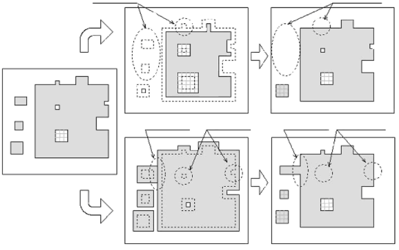
Noise is eliminated by performing compression processing after expansion processing
has been carried out (See
Figure 144
).
2) “Cut Outer Noise”
Noise is eliminated by executing expansion processing after compression processing
has been carried out (See
Figure 144
).
Noises of inside and outside of the component can be eliminated by using both “Cut
Inner Noise” and “Cut Outer Noise“ functions.
The processing results vary depending on the order in which the noise elimination
functions are executed. The execution sequence of the functions should be selected
according to need.
Figure 144
<Expansion processing>
The bottom figure in the middle in
Figure 144
shows the result after expanding the image on
the left by 1 pixel. As shown in this example, if the gray area is expanded by 1 pixel, a section
consists of two or less pixels in the component is embedded.
Multiple pixels can be specified for expansion, so the section containing the multiple pixels
(noise) is embedded. Performing compression processing following the expansion processing
produces an image without the noise. (See the bottom figure on the right in
Figure 144
).
Dele
ted
Compressed
Expand
Deleted
Deleted
Deleted
Expand
Compressed
Connected
Connected
Noise
elimination
outside the component
Noise
elimination
inside the component
174/178
IM-SMT-VSNDIC-0002-000
<Compression processing>
The top figure in the middle in
Figure 144
shows the result after compressing the image on the
left by 1 pixel. As shown in this example, if the gray area is compressed by 1 pixel, a section
consists of two or less pixels in the component is deleted. As multiple pixels can be
specified for compression, the section containing the multiple pixels (noise) is deleted.
Performing expansion processing following the compression processing produces an image
without the noise (See the top figure on the right in
Figure 144
).
Appendix 2. Detection level differences used to detect leads (threshold value)
This parameter is used when leads are being detected. For lead detection, scanning is
performed within the search range in order to separate the leads from the background.
During the scanning process, if there are any pixels that are brighter than the value specified
as the difference in detection level from the background density, those pixels are recognized
as leads. Consequently, setting a lower value for this parameter makes it possible to detected
dark leads. If the value is too low, however, the results are more easily affected by the noise.
Moreover, setting a larger value is more effective in terms of noise, but there is a greater
possibility of error in detecting the leads themselves.
The recognition conditions should be set in such a way that the illumination produces a
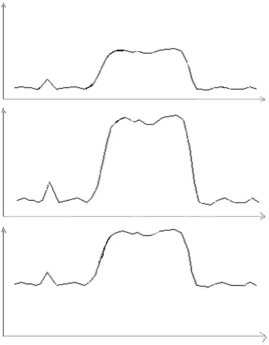
strong contrast between the background and the leads. In the figure below, the illumination
has been set to maximize the difference in levels between the lead section and the
background section. If the lighting is too dark, the brightness of the lead itself decreases,
and there will be no contrast. Conversely, if the lighting is too bright, the brightness of the
background increases, eliminating contrast between the background and the lead.
Figure 145
Brightness
Brightness
Brightness
With dark lighting
With appropriate
lighting
With bright lighting
175/178
IM-SMT-VSNDIC-0002-000
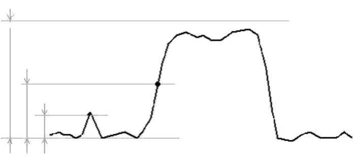
For example, if the brightness is distributed as shown in
Figure 146
along the line being
scanned, the leads can be detected correctly with the difference in detection levels (threshold
A), but with detection level difference B, reaction to the noise can be seen. With detection
level difference C, the leads cannot be detected at all.
Figure 146
Consequently, the largest possible value should be set as the detection level difference
in order not to detect the noise within a range in which there is no error in lead detection.
Normally, a value that is approximately half of the difference between the maximum
luminance and the background luminance is thought to be appropriate.
In a search for the appropriate value, the center value of the range where recognition is
performed successfully is obtained as the set value, while changing the combination of the
illumination level and the detection level difference.
However, as searches for the appropriate value are conducted only on one component,
disparities between components are not taken into consideration.
Appendix 3. Creating simple data in the special recognition modes
Some recognition modes provide modes called “special recognition modes”. These are used
to recognize components that cannot be recognized with the standard settings. In this case, a
special mode is also used for the component data settings.
All of the setting items can be entered in this mode, in other words, it is necessary to set all of
the required setting items manually. In order to minimize the manual work, the data can be
created using the standard procedure described below and then the recognition mode
changed in order to eliminate delays in creating the data.
For example, when the SOP data is created in a normal manner by using the Special 1
algorithm for SOP recognition, the following changes are made:
Alignment Group : Special component ( IC component)
Alignment Type : Special shape ( SOP)
Then the following are set in order to eliminate delays in creating the data:
Algorithm : Special 1
Base Alignment Type : SOP
The data for the lead length, Lead Width, Lead Pitch and reference lead position (Find Pos)
can be created automatically by entering the data as usual.
After that, the data set automatically is retained just as it is, and the correction is required to
be made only for the necessary items.
Detection level difference C
Detection level difference A
Detection level difference B
Background intensity
Brightness distribution on the scan line