MR8740T_user_manual_eng_20191016H.pdf - 第174页
169 Operators of W aveform Calculation and Calculation Results 8.3 Operators of W aveform Calculation and Calculation Results b i : i th data point of calculation results, d i : i th data point acquired across the source…
168
Conguring Waveform Calculation Settings
Calculation result
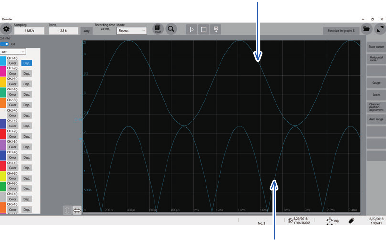
Example: To display the waveform processed through the absolute value calculation using a
waveform acquired across CH1_1
Arithmetic expression Z1= ABS(CH(1,1))
Waveform acquired across CH1-1
Calculated absolute value Z1

169
Operators of Waveform Calculation and Calculation Results
8.3 Operators of Waveform Calculation and
Calculation Results
b
i
:
i
th data point of calculation results,
d
i
:
i
th data point acquired across the source channel
Waveform calculation
type
Description
Four arithmetic
operations (+, −, ×, ÷)
Makes calculations using operators specied from the four arithmetic operations, which
consists of addition (+), subtraction (−), multiplication (×), and division (÷). Multiplication
signs (×) and division signs (÷) are represented as asterisks (*) and slashed (/),
respectively.
Absolute value (ABS)
b
i
= | d
i
| (i = 1, 2, . . . , n)
Exponent (EXP)
b
i
= exp (d
i
) (i = 1, 2, . . . , n)
Common logarithm
(LOG)
With
d
i
> 0 b
i
= log
10
d
i
With
d
i
= 0 b
i
= −∞
(Outputs overowing values)
With
d
i
< 0 b
i
= log
10
| d
i
| (i = 1, 2, . . . , n)
Note: The following expressions can convert common logarithms into natural
logarithms.
InX = log
e
X = log
10
X / log
10
e
1 / log
10
e ≈ 2.30
Square root
For
d
i
≥ 0 b
i
= √d
-
i
With
d
i
< 0 b
i
= −√
|
d
-
i
| (
i = 1, 2, . . . , n)
Cube root (CBR)
=
√
3
Moving average (MOV)
For this function, specify the number of moving points at the second parameter
k
.
When
k
is an odd number When
k
is an even number
−1
−1
∑
d
t
( = 1, 2, . . . , n)
d
t
. . . ,
d
t
:
t
th data point acquired across the source channel
k
: Number of moving point (1 to 5000)
Specify the constant
k
following a comma. Example: To calculate 100-point moving
averages of the Z1 data. MOV(Z1,100)
For each
k
/2 points of data at the beginning and end of the calculation interval, the
instrument makes calculations by plugging in zero for data-missing parts
Parallel move in the
time axis direction
(SLI)
For this function, specify the number of moving points at the second parameter k.
The instrument yields waveforms parallel moving in the time axis direction by the
specied number of points.
b
i
= d
i−k
(i = 1, 2, . . . , n)
k
: Number of moving point (−5000 to 5000)
Specify the constant
k
following a comma. Example: To move data Z1 by 100 points
SLI(Z1,100)
Note When waveforms are parallelly moved, the non-data parts at the beginning or
end of the calculation interval measure a voltage of 0 V.
Sine (SIN)
b
i
= sin(d
i
) (i = 1, 2, . . . , n)
For the trigonometric and inverse trigonometric functions, specify numbers in radians
(rad).
Cosine (COS)
b
i
= cos(d
i
) (i = 1, 2, . . . , n)
For the trigonometric and inverse trigonometric functions, specify numbers in radians
(rad).
Tangent (TAN)
b
i
= tan(d
i
) (i = 1, 2, . . . , n)
For the trigonometric and inverse trigonometric functions, specify numbers in radians
(rad).
8
Waveform Calculation Function

170
Operators of Waveform Calculation and Calculation Results
b
i
:
i
th data point of calculation results,
d
i
:
i
th data point acquired across the source channel
Waveform calculation
type
Description
Arc sine (ASIN)
With
d
i
> 1 b
i
= π / 2
With
−1 ≤ d
i
≤ 1 b
i
= arcsin(d
i
)
With
d
i
< −1 b
i
= −π / 2 (i = 1, 2, . . . , n)
For the trigonometric and inverse trigonometric functions, specify numbers in radians
(rad).
Arc cosine (ACOS)
With
d
i
> 1 b
i
= 0
With
−1 ≤ d
i
≤ 1 b
i
= arccos(d
i
)
With
d
i
< −1 b
i
= π (i = 1, 2, . . . , n)
For the trigonometric and inverse trigonometric functions, specify numbers in radians
(rad).
Arc tangent (ATAN)
b
i
= arctan(d
i
) (i = 1, 2, . . . , n)
For the trigonometric and inverse trigonometric functions, specify numbers in radians
(rad).
Arc tangent 2
(ATAN2(y, x))
Responses arc tangent of (
y / x
) in the range of [
−π
,
π
]. Specify numbers in radians (rad).
ATAN2(y, x) =
With
x ≥ 0 ATAN( y / x )
With
x < 0
and
y ≥ 0 ATAN( y / x ) + π
With
x < 0
and
y < 0 ATAN( y / x ) − π
1st-order differential
(DIF)
2nd-order differential
(DIF2)
The instrument makes 1st-order differential and 2nd-order differential calculations using
5th-order Lagrange interpolation formula to obtain 1-point data from 5-point values that
includes before and after the point.
The instrument differentiates data
d
1
to
d
n
considering them as the corresponding data
for the sampling time
t
1
to
t
1
.
Note If the instrument differentiates a waveform that oscillates slowly, calculation results
vary signicantly.
In such a case, raise the second parameter of the function.
The following expressions hold provided the second parameter equals one.
Arithmetic expressions of 1st-order differential
Point
t
1
b
1
= (−25d
1
+ 48d
2
− 36d
3
+ 16d
4
− 3d
5
) / 12h
Point
t
2
b
2
= (−3d
1
− 10d
2
+ 18d
3
− 6d
4
+ d
5
) / 12h
Point
t
3
b
3
= (d
1
− 8d
2
+ 8d
4
− d
5
) / 12h
↓
Point
t
i
b
i
= (d
i−2
− 8d
i−1
+ 8d
i+1
− d
i+2
) / 12h
↓
Point
t
n−2
b
n−2
= (d
n−4
− 8d
n−3
+ 8d
n−1
− d
n
) / 12h
Point
t
n−1
b
n−1
= (−d
n−4
+ 6d
n−3
− 18d
n−2
+ 10d
n−1
+ 3d
n
) / 12h
Point
t
n
b
n
= (3d
n−4
− 16d
n−3
+ 36d
n−2
− 48d
n−1
+ 25d
n
) / 12h
b
1
through
b
n
: Calculation result data
h = Δt
: Sampling interval
Arithmetic expressions of 2nd-order differential
Point
t
1
b
1
= (35d
1
− 104d
2
+ 114d
3
− 56d
4
+ 11d
5
) / 12h
2
Point
t
2
b
2
= (11d
1
− 20d
2
+ 6d
3
+ 4d
4
− d
5
) / 12h
2
Point
t
3
b
3
= (−d
1
+ 16d
2
− 30d
3
+ 16d
4
− d
5
) / 12h
2
↓
Point
t
i
b
i
= (−d
i-2
+ 16d
i−1
− 30d
i
+ 16d
i+1
− d
i+2
) / 12h
2
↓
Point
t
n−2
b
n−2
= (−d
n−4
+ 16d
n−3
− 30d
n−2
+ 16d
n−1
− d
n
) / 12h
2
Point
t
n−1
b
n−1
= (−d
n−4
+ 4d
n−3
+ 6d
n−2
− 20d
n−1
+ 11d
n
) / 12h
2
Point
t
n
b
n
= (11d
n−4
− 56d
n−3
+ 114d
n−2
− 104d
n−1
+ 35d
n
) / 12h
2