IPC-TM-650 EN 2022 试验方法--.pdf - 第465页
IPC-TM-650 Page 8 of 1 1 Number 2.5.5.5.1 Revision Subject Stripline Test for Complex Relative Permittivity of Circuit Board Materials to 14 GHz Date 3/98 An alternate method for trimming the copper strip is to use a sha…
available based on equation (1). Note that the de-embedded
insertion loss is defined with a reference impedance of the
transmission line.
1.3 General Calibration/de-embedding Methods to Set
up Correct Reference Plane for Printed Board Conduc-
tor Insertion Loss Characterization
As mentioned earlier,
there are existing calibration/de-embedding methods for gen-
eral purpose interconnect characterization to move the cali-
bration reference plane to printed board interfaces. These
methods are validated by the industry, and therefore included
herein, although they are either more complicated or costly
than the Eigen-value based method.
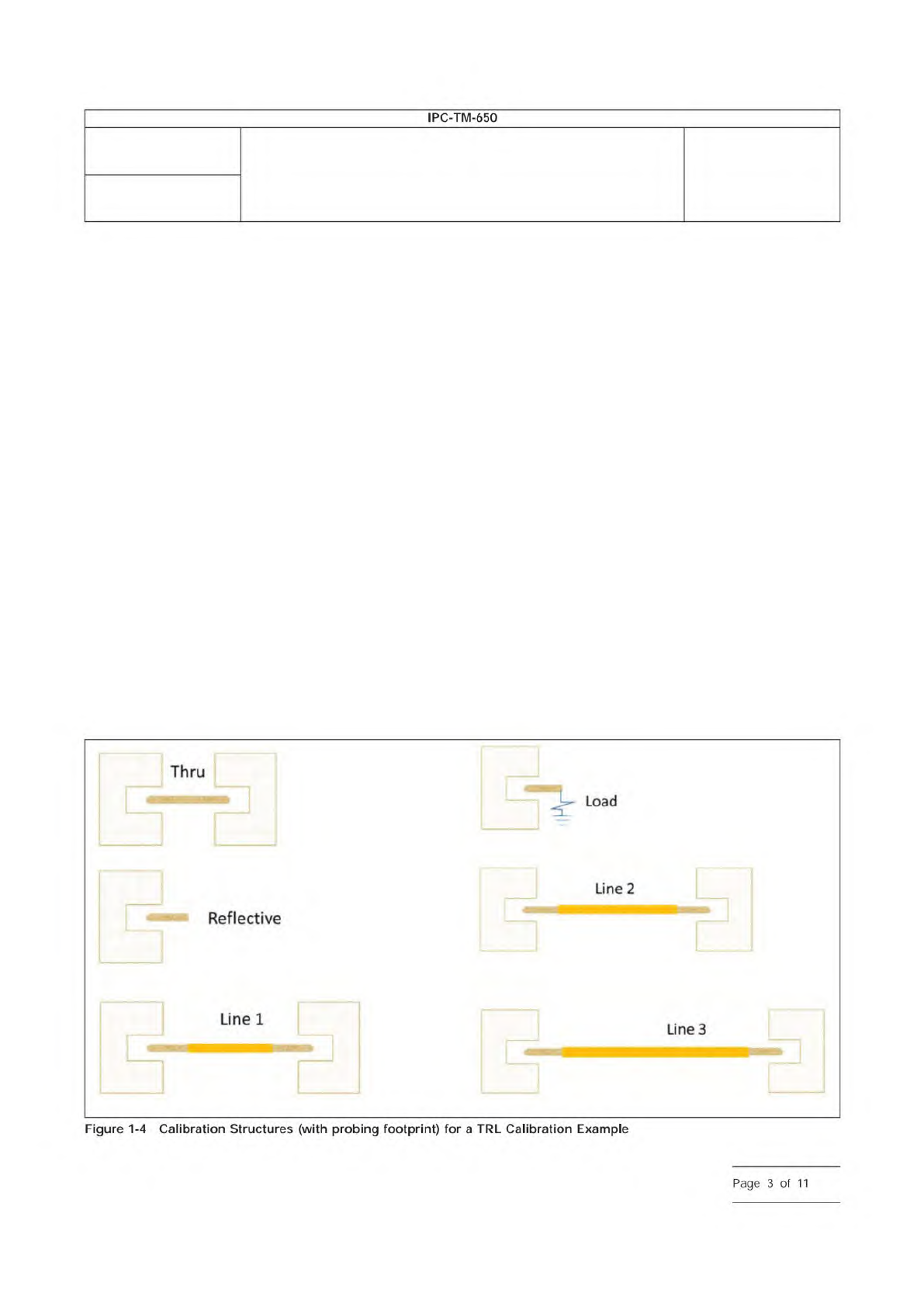
1.3.1 TRL Calibration
The TRL (and its variants such as
LRM) method [7] is a general approach to move the calibra-
tion reference plane from the coaxial connector to printed
board interfaces. Figure 1-4 shows the typical calibration
structures for a TRL calibration, with microwave probe foot-
print (with single-ended probing as an example). The TRL cali-
bration technique only relies on the characteristic impedance
of the transmission line and does NOT need the parasitics of
Reflective Standard to be known, nor propagation delay of
Line. A typical TRL calibration structure may also include a
Load structure that works only at very low frequencies, and
additional Line structures to cover a wide frequency range.
Most VNAs offer TRL calibration options, please refer to the
manual or application note for your specific equipment to per-
form a TRL calibration.
TRL calibration has been widely used in the industry since the
technique no longer requires accurate calibration termination
standards. This overcomes the difficulties of SOLT calibration,
and the reference plane can be moved to the printed board.
However, there are still some disadvantages to the TRL cali-
bration. For example, there are many components of the cali-
bration standard to handle. This takes substantial printed
board area and requires tedious calibration process in the lab,
while being prone to the operator error. Additionally, the TRL
technique requires accurate characteristic impedance specifi-
cation for the line standard, which is problematic to determine
in a dispersive environment.
1.3.2 2X-Thru De-embedding
In the last decade, the
2X-thru de-embedding methodology is gaining popularity due
to its simplicity of test fixture design and de-embedding pro-
cedures [8]. In contrast to the TRL calibration technique,
which requires measurement of multiple structures as shown
in Figure 1-4, 2X-Thru De-embedding requires only one
de-embedding structure.
The basic idea of the 2X-Thru de-embedding approach is
shown in Figure 1-5. The S-parameters of the 2X-thru
IPC-25514-1-4
Number
2.5.5.14
Subject
Measuring High Frequency Signal Loss and Propagation on
Printed Boards with Frequency Domain Methods
Date
02/2021
Revision
IPC-TM-650
—
Thru
Reflective
Line
1
Figure
1-4
Calibration
Structures
(with
probing
footprint)
for
a
TRL
Calibration
Example
Page
3
of
11
IPC-TM-650
Page 8 of 11
Number
2.5.5.5.1
Revision
Subject
Stripline
Test
for
Complex
Relative
Permittivity
of
Circuit
Board
Materials
to
14
GHz
Date
3/98
An
alternate
method
for
trimming
the
copper
strip
is
to
use
a
sharp
scalpel.
However,
this
can
smear
the
copper
across
that
the
specimen
end
surface,
especially
with
thin
speci¬
mens,
and
may
introduce
end
fringing
errors
on
short
L
val¬
ues.
6.1.5
Fasten
the
probe
assemblies
to
the
clamped
stack
at
both
ends
so
that
the
coaxial
cable
probe
end
is
centered
on
the
stripline
resonator
center
line.
Adjust
the
assembly
so
the
contact
areas
on
the
soldered
copper
fitting
make
firm
electri¬
cal
contact
by
the
wires
to
both
top
and
bottom
copper
plates.
Figure
9
shows
by
vertical
and
horizontal
sectional
views
through
the
stripline
resonator
centerline
this
relation¬
ship
among:
•
the
copper
ground
plates
(see
5.1.2).
•
the
specimen
with
conductors
(see
3.0).
•
the
coaxial
cable
with
extended
center
conductor
end
(see
5.2.1).
•
the
copper
fitting
(see
5.2.2)
soldered
to
the
coaxial
cable.
•
the
wire
connection
(see
5.2.3).
For
the
purpose
of
this
method
horizontal
orientation
is
paral¬
lel
to
the
plane
of
the
specimen
surface
in
the
fixture.
See
three
requirements
under
5.2.4.
6.1.6
Adjust
the
position
of
the
coaxial
cable
probe
ends
so
the
air
gaps
they
form
with
the
stripline
resonator
element
are
equal.
This
may
be
done
with
the
help
of
a
network
analyzer
set
for
lowest
frequency
by
adjusting
the
gaps
smaller
until
each
causes
a
sudden
shift
in
reflected
or
transmitted
power,
then
adjusting
them
back
to
a
small
gap
value,
equal
on
both
ends.
6.1.7
With
the
probe's
longitudinal
position
set
to
a
small
air
gap
such
as
0.05
mm,
use
an
appropriate
means
with
the
electronic
instrumentation
to
identify
the
approximate
location
of
the
lowest
resonant
frequency
(the
fundamental
where
the
resonator
length
is
half
the
wavelength
in
the
material
being
tested)
and
a
series
of
resonances
(harmonics)
up
to
the
high¬
est
frequency
of
interest.
Ideally
harmonic
resonances
occur
at
each
integer
multiple
of
the
fundamental
resonance.
The
integer
multiples
are
the
values
of
n
in
formula
1
of
section
7.1
.
Select
which
of
these
resonances
will
be
measured
as
discussed
in
section
6.3,
6.4,
or
6.5.
6.2
Adjustment
of
Air
Gap
for
Each
Resonance
Before
the
measurement
at
each
resonance,
adjust
the
air
gaps
at
each
probe
an
equal
amount
to
get
the
dB
insertion
loss
at
the
maximum
transmission
to
a
recommended
value
between
49.5
and
51.5
dB.
As
resonant
frequency
is
increased
from
resonance
to
resonance
for
a
given
specimen,
the
gap
required
for
a
nominal
50
dB
insertion
loss
at
resonance
tends
to
increase.
A
high
value
dB
minimizes
the
correction
for
unloaded
Q
and
makes
this
correction
less
sensitive
to
poor
data
on
the
baseline
dB
of
the
instrumentation.
Too
high
a
dB
value
will
put
the
measurements
down
in
the
noise
region
of
the
instrumentation,
making
results
less
certain
and
less
reproducible.
6.3
Manual
Measurement
of
the
Specimen
The
follow¬
ing
procedure
is
most
applicable
where
only
equipment
as
described
in
4.1
is
available.
The
equipment
of
4.2
could
also
be
operated
manually.
6.3.1
The
resonant
frequency
shall
be
found
by
scanning
frequency
over
the
expected
transmission
range
of
the
test
resonator.
The
frequency
shall
be
precisely
adjusted
to
get
a
maximum
reading
of
power
in
dB.
6.3.2
Determine
half
power
points
by
adjusting
frequency
to
give
three
dB
readings
both
above
and
below
the
maximum
transmission
frequency.
Measure
each
frequency
with
the
fre¬
quency
meter
and
record
the
results:
•
f1
-
3
dB
down,
below
the
maximum
transmission
fre¬
quency.
•
f2
-
3
dB
down,
above
the
maximum
transmission
fre¬
quency.
6.4
Automated
Measurement
of
the
Specimen
For
an
automated
system
to
be
used
in
performing
the
measure¬
ment,
computer
software
is
needed
that
will
collect
paired
values
of
frequency
and
transmitted
power.
From
this
data,
the
frequency
for
maximum
power
transmission
and
the
fre¬
quencies
of
the
half
power
points
are
determined.
The
com¬
puter
program
may
optionally
include
computation
of
permit¬
tivity
and
loss
tangent
as
described
in
section
7.0.
Results
and
collected
data
may
be
displayed
on
the
screen,
stored
in
a
disk
file,
sent
to
a
printer,
or
any
combination
of
these.
In
one
possible
mode
of
operation,
with
the
equipment
described
in
4.2,
the
sequence
of
steps
described
in
6.4.1
through
6.4.4
is
performed
as
many
times
as
necessary
to
get
enough
data
to
complete
the
test
procedure.
The
computer
is
designated
as
the
controller
on
the
GPIB.
z
IPC-TM-650
Page 9 of 11
Number
2.5.5.5.1
Revision
Subject
Stripline
Test
for
Complex
Relative
Permittivity
of
Circuit
Board
Materials
to
14
GHz
Date
3/98
6.4.1
The
computer
sets
the
sweeper
to
a
selected
carrier
wave
frequency
without
an
AM
or
FM
audio
signal
and
to
a
desired
output
power
level,
such
as
10
dBm.
6.4.2
The
same
frequency
is
given
to
the
synchronizer
with
instructions
to
lock the
frequency
of
the
sweeper
to
the
speci¬
fied
value.
6.4.3
The
computer
checks
the
synchronizer
for
status
until
the
status
value
indicates
the
frequency
is
locked.
6.4.4
The
power
meter
reading
is
obtained
by
the
computer.
Since
it
takes
a
finite
amount
of
time
for
the
power
sensor
to
stabilize,
either
a
delay
is
used
or
the
reading
may
be
taken
repeatedly
until
consecutive
readings
meet
a
given
require¬
ment
for
stability.
6.5
Use
of
the
Network
Analyzer
for
Measurement
of
the
Specimen
An
automated
network
analyzer
may
be
used
either
by
operating
the
front
panel
controls
manually
or
under
computer
control
with
suitable
specialized
software.
The
fixture
with
the
specimen
is
connected
by
test
cables
and
adapters
as
a
device
under
test.
Set
up
the
instrument
so
the
Cartesian
screen
display
shows
the
S21
parameter,
the
transmission/incident
power
ratio,
in
negative
dB
vertical
scale
units
versus
frequency
on
the
horizontal
scale.
Select
the
start
and
stop
frequency
range
to
sweep
across
the
resonance
peak
and
at
least
3
dB
below
the
peak.
Adjust
the
start
and
stop
frequency
values
as
narrowly
as
possible,
but
still
include
the
resonant
peak
and
the
portions
of
the
response
curve
on
both
sides
of
it
that
extend
3
dB
downward.
6.5.1
The
first
option
is
to
get
the
three
points
(fr,
f
〕
and
f2)
as
described
in
6.3
or
6.4.
Determine
the
resonant
dBr
and
frequency
fr
values
for
the
highest
point
(maximum)
on
the
response
curve.
With
manual
operation,
instrument
program
features
may
be
available
to
do
this
very
quickly.
On
the
response
curve
to
the
left
and
right
of
fr,
locate
the
%
,
dB〕
and
f2,
dB2
points
as
near
as
possible
to
3
dB
below
dBr.
These
may
then
be
used
in
the
calculations
shown
in
7.2.
6.5.2
A
second
option
requires
a
computer
external
to
the
instrument.
Collect
from
the
network
analyzer
all
of
the
f,
dB
data
points
represented
by
the
response
curve
between
dB〕
and
f2,
dB2
and
apply
non-linear
regression
analysis
tech¬
niques
to
determine
statistically
values
for
Q,oaded)
fr
and
dBr
that
best
fit
the
f”
dB,
paired
data
points
to
the
formula.
dBj
=
dB「
-
10
loge(10)
loge
(1+4
Qloaded2
(f"
fr
-
1)2)
[1]
where
10
loge(1
0)
is
the
constant
for
converting
from
loge
to
dB.
This
formula
may
be
derived
from
formula
5
with
the
rea¬
sonable
assumption
that
fr
-
j
equals
f2
-
fr.
The
statistically
derived
values
for
fr
and
Q
would
then
be
used
in
formulas
2
of
section
7.1,
formula
3
of
section
7.2,
and
formula
6
of
sec¬
tion
7.3
respectively.
This
has
been
found
to
fit
the
collected
data
points
very
well
at
all
regions
across
the
entire
&
to
f2
range.
It
is
a
simplified
version
of
the
non-linear
regression
method
for
complex
S21
parameters
described
by
Vanzura4.
7.0
Calculations
7.1
Stripline
Permittivity
Use
special
care
to
assign
the
correct
n
value
for
each
resonance
measured.
At
resonance,
the
electrical
length
of
the
resonator
circuit
is
an
integral
number
of
half
wavelengths.
The
effective
stripline
permittivity,
耳,
can
be
calculated
from
the
frequency
of
maxi¬
mum
transmission
as
follows:
加二
[n
C
/
(2
fr(L
+
AL))]2
[2]
where
n
is
the
number
of
half
wavelengths
along
the
resonant
strip
of
length
L
in
mm,
AL
is
the
total
effective
increase
in
length
of
the
resonant
strip
due
to
the
fringing
field
at
the
ends
of
the
resonant
strip,
C
(the
speed
of
light)
is
2.9978
1011
mm/s,
and
fr
in
Hz
(or
cycles/s)
is
the
measured
resonant
(maximum
transmission)
frequency.
The
resonator
ends
coincide
with
the
end
edges
of
both
the
dielectric
and
the
ground
planes.
The
relative
fringing
field
at
the
ends
becomes
extremely
small.
It
has
been
the
practice
with
this
method
to
ignore
this
fringing
field
and
consider
the
AL
value
to
be
zero
in
the
calculation
of
stripline
permittivity.
7.2
Calculation
of
Effective
Dielectric
Loss
Tangent
tan
6
=
1/Qunloaded
-
1/Qc
where:
1/QC
is
the
loss
factor
of
the
conductor
1/Qunioaded
is
the
total
loss
factor
of
the
unloaded
resonator
due
only
to
the
dielectric,
copper,
and
copper-dielectric
inter¬
face,
and
does
not
include
loss
due
to
coupling
of
the
probes.
7.2.1
The
resonator
loss
factor
The
measurement
of
the
resonance
gives
a
value
for
the
loss
factor
of
the
resonator
with
loading
due
to
probe
coupling
(1/Q,oaded).