MR8740、MR8741_user_manual_eng_20191016H.pdf - 第248页
10.2 Settings for Waveform Calcula tion 236 W aveform Calcu- lation Example Calculate the RMS waveform from the inst antaneous waveform The RMS values of the waveform inp ut on Channel 1 are calculated and dis- played. T…
10.2 Settings for Waveform Calculation
235
9
Chapter 10 Waveform Calculation Functions
10
10.2.3 Changing the display method for calculated
waveforms
Procedure
To open the screen: Right-click and select [STATUS] [Wave Calc] sheet
1
Enable waveform display, and display color
Move the flashing cursor to the [Wave] column.
Select
2
Select a method to set scaling
Move the flashing cursor to the [Scale] column for the Calculation No.
to be set.
Select
3
Set the upper and lower limits of the display range (when
[Manual] is selected)
Select [Lower] and [Upper].
Select an entry method and enter the limit values.
Entry range: -9.9999E+29 to +9.9999E+29
See: "7.1.3 Alphanumeric Input" (p.141)
4
Specify the physical units
Move the flashing cursor to the [Unit] column.
Select an entry method and enter the physical units.
See: "7.1.3 Alphanumeric Input" (p.141)
5
Select the graph to be displayed.
(When split screen ([Format] item on the [Status] sheet) is
[Dual] or higher)
Move the flashing cursor to the [Graph] column and select the graph
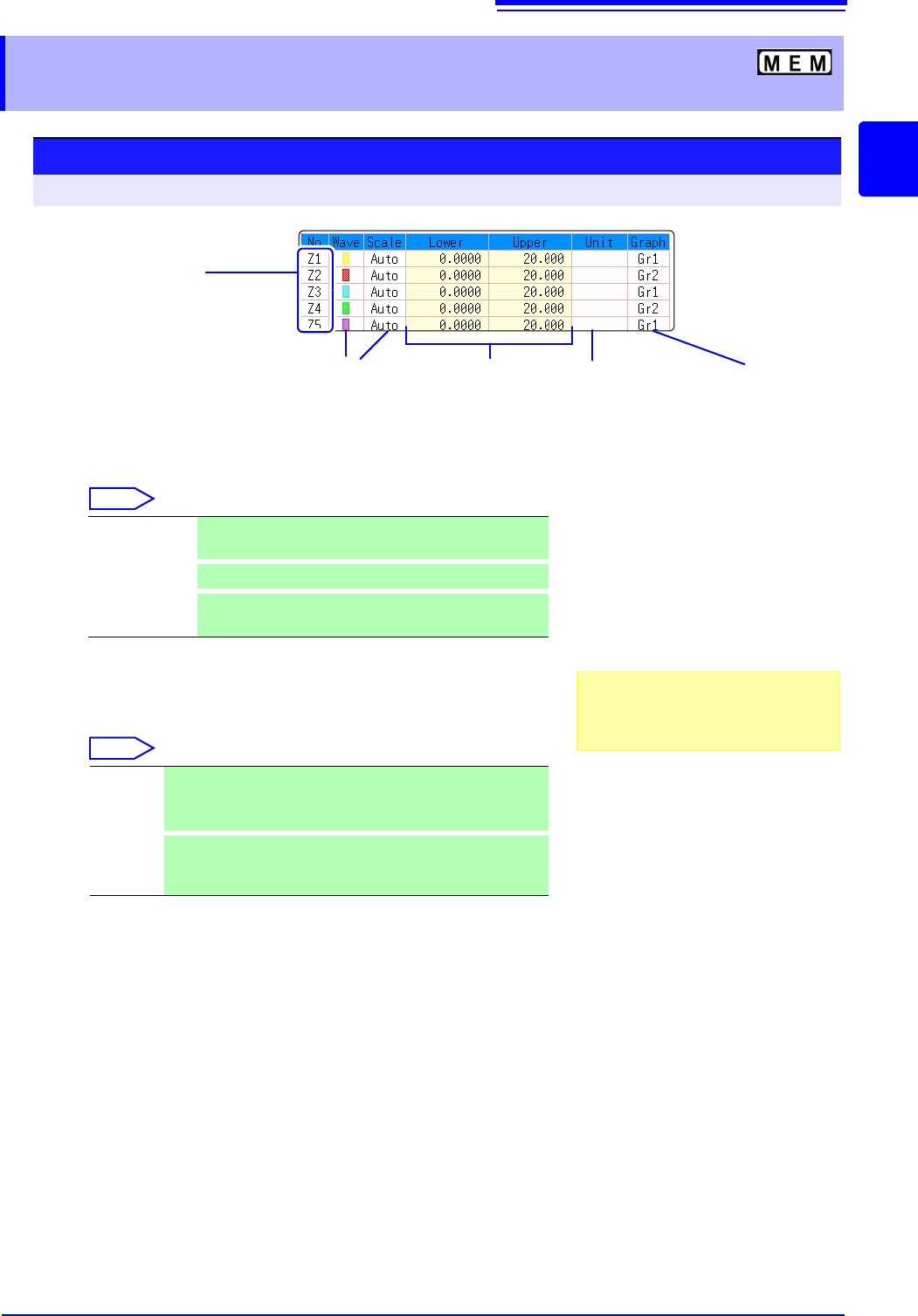
b
Waveform
color
Upper and
lower limits
Displayed
measurement units
Display range
setting method
Calculation No.
To copy settings
between Calculation Nos.:
Click the calculation No.
12 43
Graph to
display
6
On-Off Set On to display the waveform of the flashing cursor
column (default setting). Set to Off to hide display.
Select the waveform color.
All On-Off
Select On to display all waveforms. Select Off to hide all
waveforms.
Auto Automatically sets the display range of the vertical axis. (After
calculation, the upper and lower limits are obtained from the
results, and set automatically.)
Manual
Upper and lower limits of the vertical axis display range are
entered manually.
A shorter calculation time than with Auto is possible.
Depending on calculation results, auto-
matic scaling settings may be unsatisfac-
tory, in which case the limits must be
entered manually.
10.2 Settings for Waveform Calculation
236
Waveform Calcu-
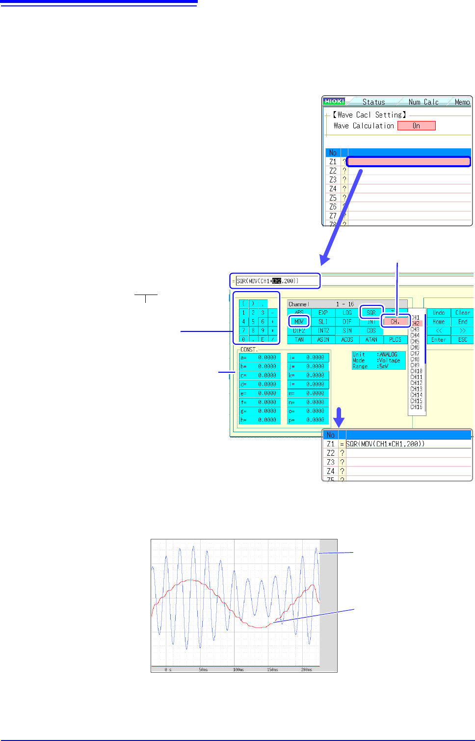
lation Example
Calculate the RMS waveform from the instantaneous waveform
The RMS values of the waveform input on Channel 1 are calculated and dis-
played. This example describes the calculation of waveform data measured for
one cycle over two divisions.
1
3
1
Enable the Waveform Calculation function.
Move the flashing cursor to the [Wave Calculation] item,
and select [On].
2
Specify the waveform calculation range.
Move the flashing cursor to the [Calc Area] item, and select
[Whole Area].
3
Perform calculation settings.
Move the flashing cursor to the [Equation] column of No. Z1
and then select [Enter EQN].
A dialog is displayed for entering a calculation equation.
4
When finished entry, select [Confirm].
The entered equation is displayed in the [Equation] field.
5
Execute the calculations.
Click [START] to start measurement.
The calculation waveform is displayed after acquiring the input wave-
form.
It is convenient to set con-
stants beforehand on the
[CONST.] (
p.234)
Enter numerical values
and symbols
Entering the calculation equation
SQR(MOV(CH1*CH1,200))
The number of samples per cycle (1 division = 100
samples) Here, one cycle is two divisions (200
samples)
After selecting the channel num-
ber, select the [Enter Char] but-
ton.
To view calculated waveforms of loaded data, move to the [Wave Calc] sheet and select [Exec].
CH1 Waveform
Calculation waveform of
RMS values

10.3 Waveform Calculation Operators and Results
237
9
Chapter 10 Waveform Calculation Functions
10
10.3 Waveform Calculation Operators and
Results
b
i
: ith member of calculation result data, d
i
: ith member of source channel data
Waveform Calculation Type Description
Four Arithmetic Opera-
tors ( +, -, *, / )
Executes the corresponding arithmetic operation.
Absolute Value (ABS)
b
i
= | d
i
| (i = 1, 2, .... n)
Exponent (EXP)
b
i
= exp(d
i
) (i = 1, 2, .... n)
Common Logarithm
(LOG)
When d
i
> 0 , b
i
= log
10
d
i
When d
i
= 0 , b
i
= - (overflow value output)
When d
i
< 0 , b
i
= log
10
| d
i
| (i = 1, 2, .... n)
Note: Use the following equation to convert to natural logarithm calculations.
LnX = log
e
X = log
10
X / log
10
e
1 / log
10
e 2.30
Square Root (SQR)
When d
i
0 , b
i
=
When d
i
< 0 , b
i
= - (i = 1, 2, .... n)
Moving Average (MOV)
dt: t
th
member of source channel data
k : number of points to move (1 to 5000)
1 div = 100 points.
k is specified after a comma.
(Ex.) To make Z1 the moving average of 100 points: MOV(Z1,100
)
Slides waveform data
along the time axis (SLI)
Moves along the time axis by the specified distance.
b
i
= d
i
k (i = 1, 2, .... n)
k : number of points to move (-5000 to 5000)
k is specified after a comma.
(Ex.) To slide Z1 by 100 points along the time axis: SLI(Z1,100
)
Note: When sliding a waveform, if there is no data at the beginning or end of the calcula-
tion result, the voltage value becomes zero. 1 div = 100 points.
Sine (SIN)
b
i
= sin(d
i
) (i = 1, 2, .... n)
Trigonometric functions employ radian (rad) units.
Cosine (COS)
b
i
= cos(d
i
) (i = 1, 2, .... n)
Trigonometric functions employ radian (rad) units.
Tangent (TAN)
b
i
= tan(d
i
) (i = 1, 2, .... n)
where -10
b
i
10
Trigonometric functions employ radian (rad) units.
Arcsine (ASIN)
When d
i
> 1, b
i
=
/ 2
When -1
d
i
1, b
i
= asin(d
i
)
When d
i
< 1, b
i
= -
/ 2
Trigonometric functions employ radian (rad) units.
8
d
i
d
i
bi
1
k
---
dt
ti
k
2
---
–=
i
k
2
---+
=
(i = 1, 2, .... n)
When k is odd number:
bi
1
k
---
dt
ti
k
2
---
–1+=
i
k
2
---+
=
(i = 1, 2, .... n)
When k is even number: