MR8740、MR8741_user_manual_eng_20191016H.pdf - 第412页
Appendix 4 FFT Definitions A 16 Aliasing ______________________________________________________ When the frequency of a signal to be m easur ed is higher than the samp ling rate, the observed frequen cy is lower than tha…
Appendix 4 FFT Definitions
A15
Appendix
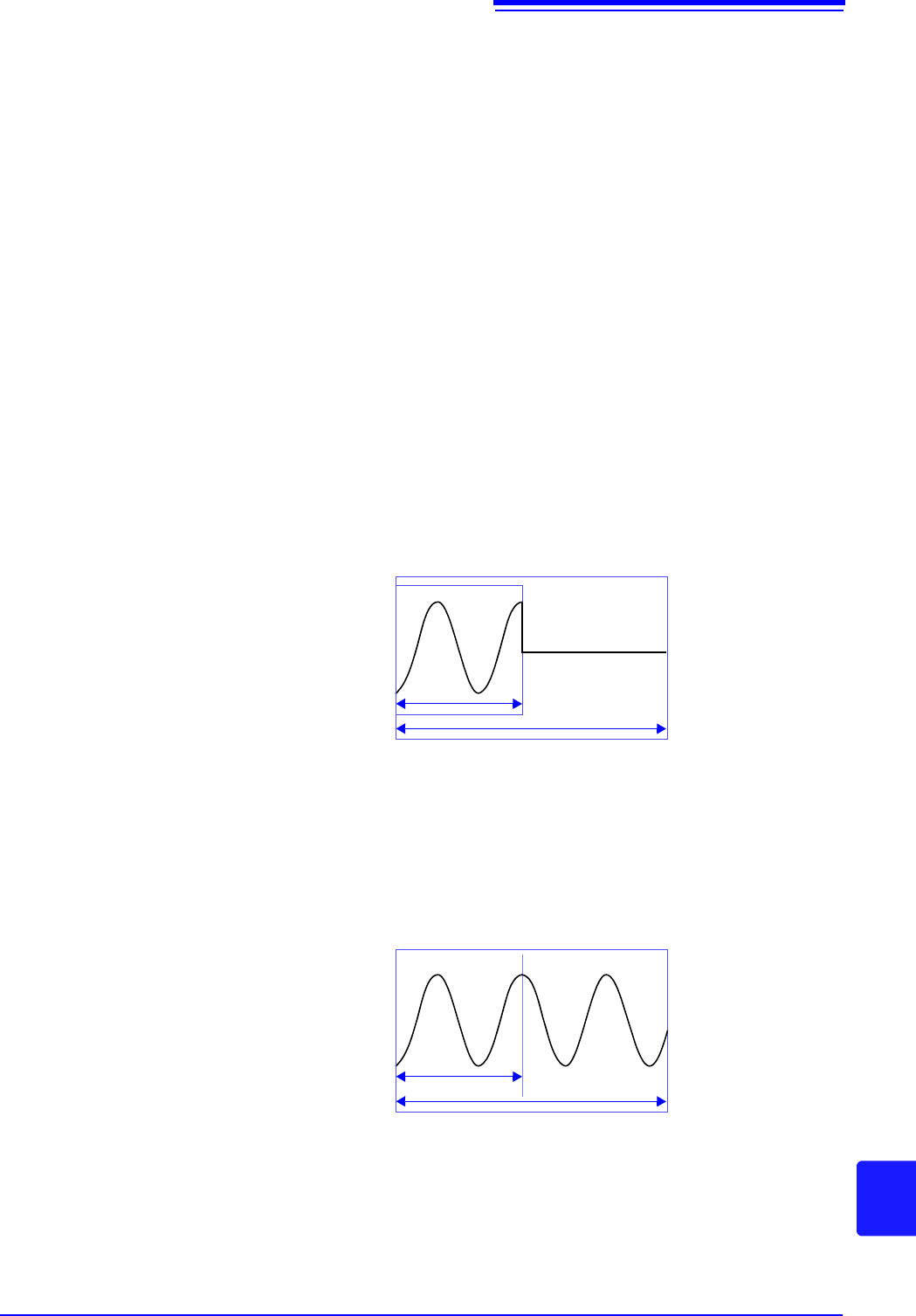
Number of Analysis Points_______________________________________
The FFT functions of this instrument can perform frequency analysis of time-
domain waveforms consisting of 1000, 2000, 5000, or 10,000 points. However,
when the following conditions are satisfied, previously analyzed data can be
reanalyzed with a different number of analysis points.
A. When measurements are made with the averaging function disabled (Off)
B. When measurements are made with the averaging function enabled for time-
domain averaging (simple or exponential).
When the number of analysis points at measurement time is N
1
and the number
of analysis points is changed to N
2
after measurement, the instrument performs
as follows.
(1) When N
1
< N
2
• Because not enough data has been collected, zero is inserted for time after
the end of the measured waveform.
• The window function applies only to the N
1
segment.
• Frequency resolution is increased. For example, if N
1
= 1000 and N
2
= 2000,
frequency resolution is doubled.
• The average energy of the time-domain waveform is reduced, so the ampli-
tude of the linear spectrum is also reduced.
(2) When N
1
> N
2
• The specified (N
2
) segment is extracted from the head of the (N
1
) data.
• The window function applies only to the N
2
segment.
• Frequency resolution is decreased. For example, if N
1
= 2000 and N
2
= 1000,
frequency resolution is halved.
• The average energy of the time-domain waveform is unchanged, so the
amplitude of the linear spectrum is not significantly affected.
N
1
N
2
N
1
N
2
Appendix 4 FFT Definitions
A16
Aliasing ______________________________________________________
When the frequency of a signal to be measured is higher than the sampling rate,
the observed frequency is lower than that of the actual signal, with certain fre-
quency limitations. This phenomena occurs when sampling occurs at a lower fre-
quency than that defined by the Nyquist-Shannon sampling theorem, and is
called aliasing.
If the highest frequency component of the input signal is f
max
and the sampling
frequency is f
s
, the following expression must be satisfied:
Therefore, if the input includes a frequency component higher than f
s
/2, it is
observed as a lower frequency (alias) that does not really exist.
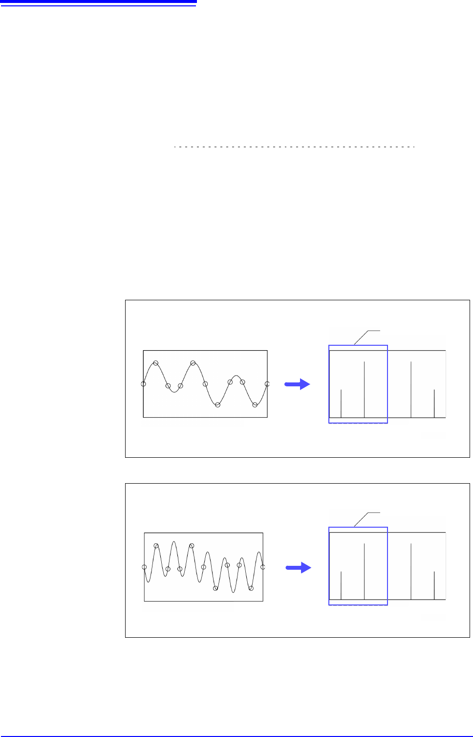
The following diagrams show the results of spectrum analysis of composite
waveforms having components of 1 kHz and 3 kHz, and of 1 kHz and 7 kHz.
If sampling frequency f
s
is 10 kHz, the spectral component of an input frequency
above 5 kHz (in this case, 7 kHz) is observed as an alias at 5 kHz or below.
In this example the difference between the 3 and 7 kHz components is indiscern-
ible.
max
2 ff
s
(10)
Composite waveform of 1 kHz and 3 kHz components sampled at 10 kHz
Time
Portion Displayed on
Screen
Spectrum
1357
Frequency
[kHz]
Composite waveform of 1 kHz and 7 kHz components sampled at 10 kHz
Time
Spectrum
Frequency
[kHz]
1357
Portion Displayed on
Screen
Appendix 4 FFT Definitions
A17
Appendix
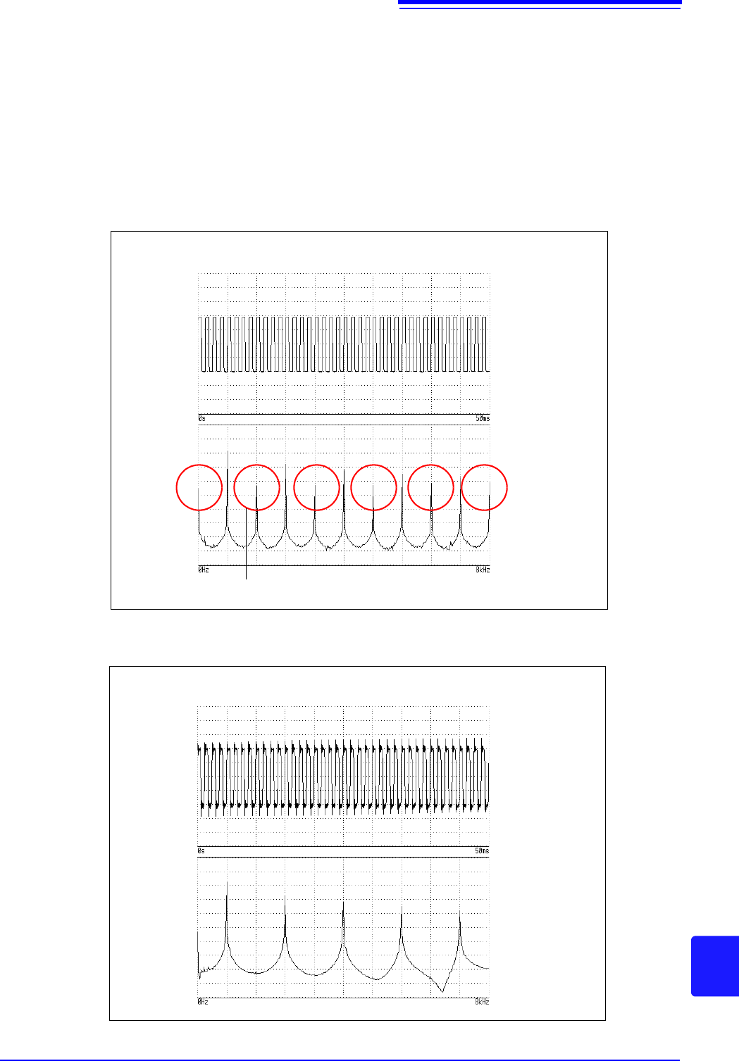
Anti-Aliasing Filters ____________________________________________
When the maximum frequency component of the input signal is higher than one-
half of the sampling frequency, aliasing distortion occurs. To eliminate aliasing
distortion, a low-pass filter can be used that cuts frequencies higher than one-
half of the sampling frequency. Such a low-pass filter is called an anti-aliasing fil-
ter.
The following figures show the effect of application of an anti-aliasing filter on a
square wave input waveform.
Non-existent frequency components are observed.
Without an anti-aliasing filter
Input time
waveform
Frequency analysis
results
With an anti-aliasing filter
Input time
waveform
Frequency analysis
results