MR8740、MR8741_user_manual_eng_20191016H.pdf - 第249页
10.3 Waveform Calculation Operators and Results 237 9 Chapter 10 W aveform Calculation Functions 10 10.3 W aveform Calculation Operators and Result s b i : ith member of calculation result data, d i : ith member of sourc…
10.2 Settings for Waveform Calculation
236
Waveform Calcu-
lation Example
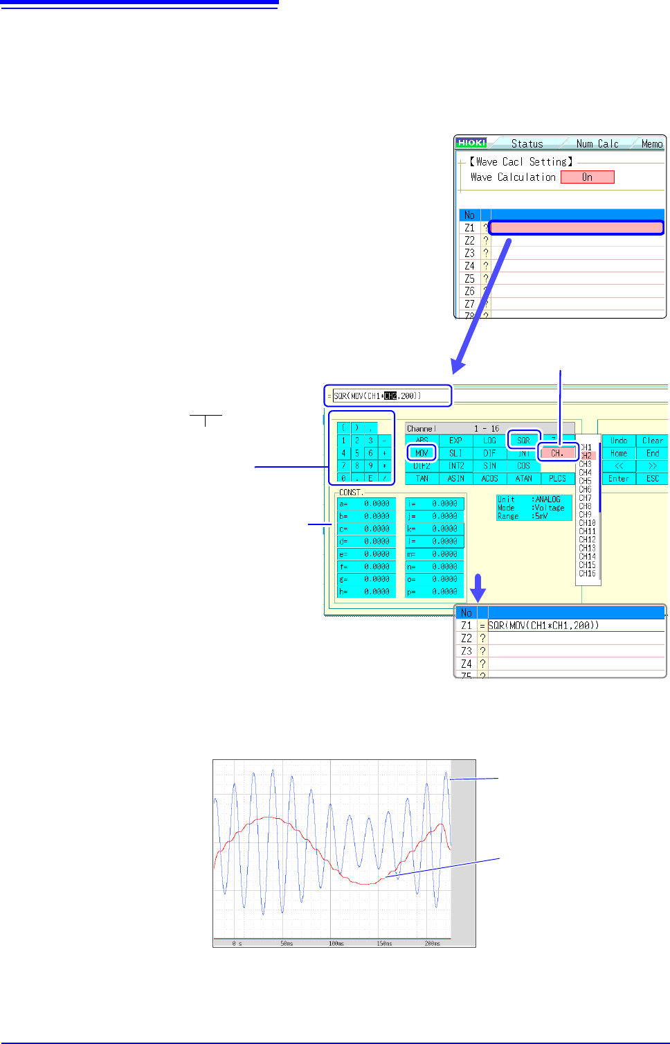
Calculate the RMS waveform from the instantaneous waveform
The RMS values of the waveform input on Channel 1 are calculated and dis-
played. This example describes the calculation of waveform data measured for
one cycle over two divisions.
1
3
1
Enable the Waveform Calculation function.
Move the flashing cursor to the [Wave Calculation] item,
and select [On].
2
Specify the waveform calculation range.
Move the flashing cursor to the [Calc Area] item, and select
[Whole Area].
3
Perform calculation settings.
Move the flashing cursor to the [Equation] column of No. Z1
and then select [Enter EQN].
A dialog is displayed for entering a calculation equation.
4
When finished entry, select [Confirm].
The entered equation is displayed in the [Equation] field.
5
Execute the calculations.
Click [START] to start measurement.
The calculation waveform is displayed after acquiring the input wave-
form.
It is convenient to set con-
stants beforehand on the
[CONST.] (
p.234)
Enter numerical values
and symbols
Entering the calculation equation
SQR(MOV(CH1*CH1,200))
The number of samples per cycle (1 division = 100
samples) Here, one cycle is two divisions (200
samples)
After selecting the channel num-
ber, select the [Enter Char] but-
ton.
To view calculated waveforms of loaded data, move to the [Wave Calc] sheet and select [Exec].
CH1 Waveform
Calculation waveform of
RMS values

10.3 Waveform Calculation Operators and Results
237
9
Chapter 10 Waveform Calculation Functions
10
10.3 Waveform Calculation Operators and
Results
b
i
: ith member of calculation result data, d
i
: ith member of source channel data
Waveform Calculation Type Description
Four Arithmetic Opera-
tors ( +, -, *, / )
Executes the corresponding arithmetic operation.
Absolute Value (ABS)
b
i
= | d
i
| (i = 1, 2, .... n)
Exponent (EXP)
b
i
= exp(d
i
) (i = 1, 2, .... n)
Common Logarithm
(LOG)
When d
i
> 0 , b
i
= log
10
d
i
When d
i
= 0 , b
i
= - (overflow value output)
When d
i
< 0 , b
i
= log
10
| d
i
| (i = 1, 2, .... n)
Note: Use the following equation to convert to natural logarithm calculations.
LnX = log
e
X = log
10
X / log
10
e
1 / log
10
e 2.30
Square Root (SQR)
When d
i
0 , b
i
=
When d
i
< 0 , b
i
= - (i = 1, 2, .... n)
Moving Average (MOV)
dt: t
th
member of source channel data
k : number of points to move (1 to 5000)
1 div = 100 points.
k is specified after a comma.
(Ex.) To make Z1 the moving average of 100 points: MOV(Z1,100
)
Slides waveform data
along the time axis (SLI)
Moves along the time axis by the specified distance.
b
i
= d
i
k (i = 1, 2, .... n)
k : number of points to move (-5000 to 5000)
k is specified after a comma.
(Ex.) To slide Z1 by 100 points along the time axis: SLI(Z1,100
)
Note: When sliding a waveform, if there is no data at the beginning or end of the calcula-
tion result, the voltage value becomes zero. 1 div = 100 points.
Sine (SIN)
b
i
= sin(d
i
) (i = 1, 2, .... n)
Trigonometric functions employ radian (rad) units.
Cosine (COS)
b
i
= cos(d
i
) (i = 1, 2, .... n)
Trigonometric functions employ radian (rad) units.
Tangent (TAN)
b
i
= tan(d
i
) (i = 1, 2, .... n)
where -10
b
i
10
Trigonometric functions employ radian (rad) units.
Arcsine (ASIN)
When d
i
> 1, b
i
=
/ 2
When -1
d
i
1, b
i
= asin(d
i
)
When d
i
< 1, b
i
= -
/ 2
Trigonometric functions employ radian (rad) units.
8
d
i
d
i
bi
1
k
---
dt
ti
k
2
---
–=
i
k
2
---+
=
(i = 1, 2, .... n)
When k is odd number:
bi
1
k
---
dt
ti
k
2
---
–1+=
i
k
2
---+
=
(i = 1, 2, .... n)
When k is even number:

10.3 Waveform Calculation Operators and Results
238
Arccosine (ACOS)
When d
i
> 1, b
i
= 0
When -1
d
i
1, b
i
= acos(d
i
)
When d
i
< -1 , b
i
=
(i = 1, 2, .... n)
Trigonometric functions employ radian (rad) units.
Arctangent (ATAN)
b
i
= atan(d
i
) (i = 1, 2, .... n)
Trigonometric functions employ radian (rad) units.
First derivative (DIF)
Second derivative (DIF2)
The first and second derivative calculations use a fifth-order Lagrange interpolation poly-
nomial to obtain a point data value from five sequential points.
d
1
to d
n
are the derivatives calculated for sample times t
1
to t
n
.
Note: Scattering of calculation results increases as input voltage level decreases. If scat-
tering is excessive, apply the moving average (MOV).
Calculation formulas for the first derivative
Point t
1
b
1
= (-25d
1
+ 48d
2
- 36d
3
+ 16d
4
- 3d
5
)/ 12h
Point t
2
b
2
= (-3d
1
- 10d
2
+ 18d
3
- 6d
4
+ d
5
)/ 12h
Point t
3
b
3
= (d
1
- 8d
2
+ 8d
4
- d
5
)/ 12h
Point t
i
b
i
= (d
i -2
- 8d
i-1
+ 8d
i+1
- d
i+2
)/ 12h
Point t
n-2
b
n-2
= (d
n-4
- 8d
n-3
+ 8d
n-1
-d
n
)/12h
Point t
n-1
b
n-1
= (-d
n-4
+ 6d
n-3
- 18d
n-2
+ 10d
n-1
+ 3d
n
)/12h
Point t
n
b
n
= (3d
n-4
- 16d
n-3
+ 36d
n-2
- 48d
n-1
+ 25d
n
)/12h
b
1
to b
n
: calculation results
h =
t : Sampling Period
Calculation formulas for the second derivative
Point t
1
b
1
= (35d
1
- 104d
2
+ 114d
3
- 56d
4
+ 11d
5
)/12h
2
Point t
2
b
2
= (11d
1
- 20d
2
+ 6d
3
+ 4d
4
- d
5
)/12h
2
Point t
3
b
3
= (-d
1
+ 16d
2
-30d
3
+ 16d
4
- d
5
)/12h
2
Point t
i
b
i
= (-d
i-2
+ 16d
i-1
- 30d
i
+ 16d
i+1
- d
i+2
)/12h
2
Point t
n-2
b
n-2
= (-d
n-4
+ 16d
n-3
- 30d
n-2
+ 16d
n-1
- d
n
)/12h
2
Point t
n-1
b
n-1
= (-d
n-4
+ 4d
n-3
+ 6d
n-2
- 20d
n-1
+ 11d
n
)/12h
2
Point t
n
b
n
= (11d
n-4
-56d
n-3
+ 114d
n-2
- 104d
n-1
+ 35d
n
)/12h
2
b
i
: ith member of calculation result data, d
i
: ith member of source channel data
Waveform Calculation Type Description