MR8740、MR8741_user_manual_eng_20191016H.pdf - 第421页
Appendix 4 FFT Definitions A 25 Appendix Oct ave Filter Characteristi cs _____________________________________ Octave filter characteristics are determin ed according to IEC61260 standard s. The figures below show these …
Appendix 4 FFT Definitions
A24
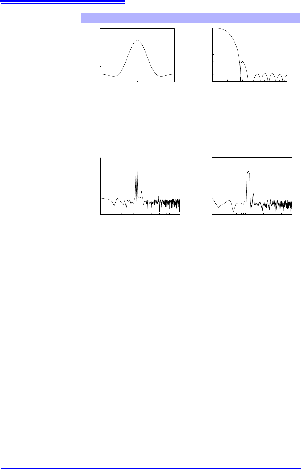
The following example shows input sine waves of 1050 and 1150 Hz analyzed
with different window functions. Because the frequencies in this example are
close to one another, a rectangular window with a narrow main lobe is able to
separate and display both frequencies, but a Hann window with a wide main lobe
displays the two as a single spectral component.
Flat top window
Time-Domain Waveform Spectrum
Analysis Using a Rectangular Window Analysis Using a Hann Window
N-10
Amplitude
0
0 2 4 6 8 10
-80
-60
-40
-20
0
Frequency (1/W)
Gain [dB]
100 500 1000 5000 10000
-100
-50
0
Frequency [Hz]
Amplitude [dB]
100 500 1000 5000 10000
-100
-50
0
Frequency [Hz]
Amplitude [dB]
Appendix 4 FFT Definitions
A25
Appendix
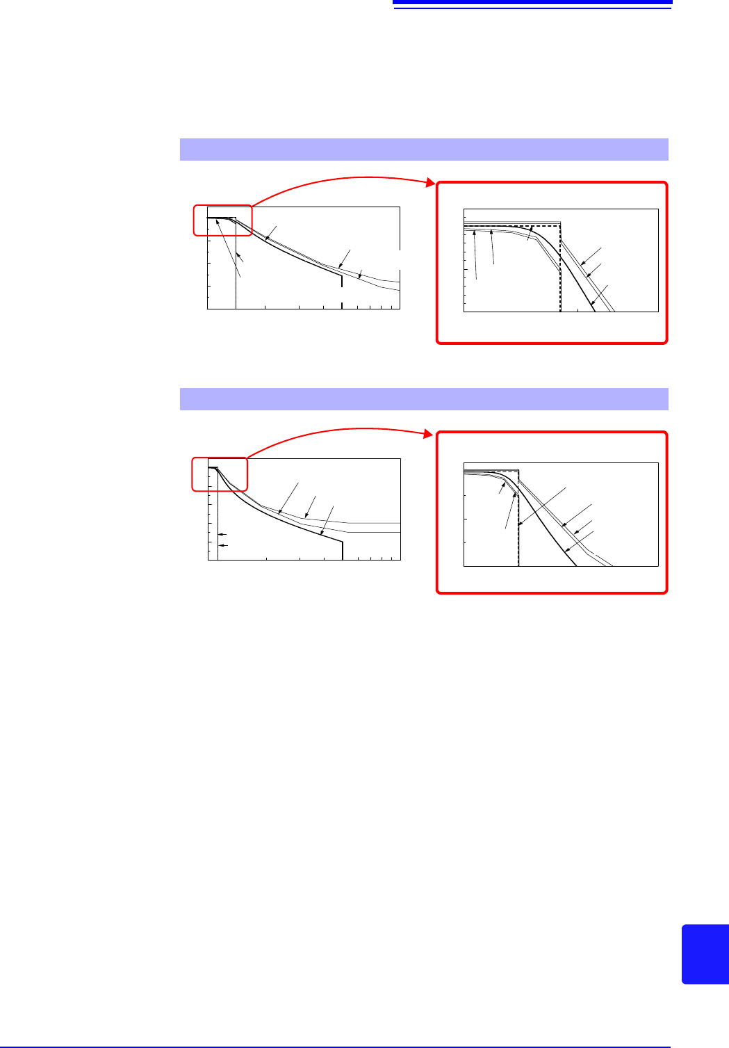
Octave Filter Characteristics _____________________________________
Octave filter characteristics are determined according to IEC61260 standards.
The figures below show these standards and the filter characteristics of this
instrument.
1/1 Octave Filter Characteristic
1/3 Octave Filter Characteristic
1 2 3 4 5 6 7 8 9 10
-80
-60
-40
-20
0
クラス1( 上限)
クラス2 (上限)
ノーマルフィルタ
規格化周波数 f/fm
ゲイン[dB]
クラス1, 2 (下限)
シャープフィルタ
Gain [dB]
1 1.5 2
-10
-5
0
クラス1 (上限)
クラス2 (上限)
ノーマルフィルタ
規格化周波数 f/fm
ゲイン[dB]
クラス1 (下限)
シャープフィルタ
クラス2 (下限)
Normalized Frequency f/fm
Normalized Frequency f/fm
Gain [dB]
Sharp
filter
Normal filter
Normal filter
Class 1 and 2 (lower limit)
Sharp filter
Class 2
(upper limit)
Class 1
(upper limit)
Class 2 (lower
limit)
Class 1
(lower limit)
Class 2
(upper limit)
Class 1
(upper limit)
1 1.5
-20
-10
0
クラス1 (上限)
クラス2 (上限)
ノーマルフィルタ
規格化周波数 f/fm
ゲイン[dB]
クラス1 (下限)
シャープフィルタ
クラス2 (下限)
1 2 3 4 5 6 7 8 9 10
-100
-80
-60
-40
-20
0
クラス1 (上限)
クラス2 (上限)
ノーマルフィルタ
規格化周波数 f/fm
ゲイン[dB]
クラス1, 2 (下限)
シャープフィルタ
Gain [dB]
Normalized Frequency f/fm
Class 1 and 2 (lower limit)
Normalized Frequency f/fm
Gain [dB]
Class 2
(upper limit)
Class 1 (upper limit)
Class 1
(lower
limit)
Class 2
(lower
limit)
Sharp filter
Normal filter
Sharp filter
Normal filter
Class 1 (upper limit)
Class 2 (upper limit)
Appendix 4 FFT Definitions
A26
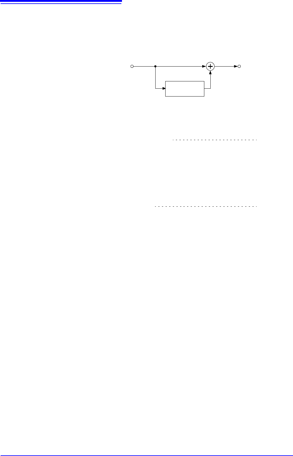
Linear Predictive Coding (LPC)___________________________________
In the following figure, linear predictive coding is implemented by passing a sam-
ple of the input signal through the prediction filter while altering the filter so as to
minimize errors in the original signal.
Given a time-discrete signal {x
t
} (t is an integer) where the input signal is sam-
pled at interval T, LPC analysis presumes the following relationship between
current sample value x
t
and the value of previous sample p.
However, is an uncorrelated random variable with average value 0 and the
dispersion .
Expression (16) shows how current sample value x
t
can be “linearly predicted”
from previous sample values. If the predicted value of x
t
is actually , expres-
sion (16) can be transformed as follows.
Here,
i
is called the linear predictor coefficient.
For LPC analysis, this coefficient is calculated using the Levinson-Durbin algo-
rithm, and a spectrum is obtained. In this instrument, the order of the coefficient
can be set from 2 to 64. Larger orders reveal fine spectral components, while
small orders reveal the overall spectrum shape.
予測フィルタ
入力信号
予測信号
誤差信号
Error Signal
Prediction Signal
Input Signal
Prediction Filter
(16)
tptpttt
xxxx
2211
}{
t
2
t
x
(17)
t
p
i
itit
t
t
xxx
1