MR8740、MR8741_user_manual_eng_20191016H.pdf - 第410页
Appendix 4 FFT Definitions A 14 Representing the ab ove relationship on a co mplex flat su rfac e produces the fol- lowing figure. Linear T ime-Invariant Syst ems _____________ _____________________ Consider a linear tim…
Appendix 4 FFT Definitions
A13
Appendix
What is FFT? __________________________________________________
FFT is the abbreviation for Fast Fourier Transform, an efficient method to calcu-
late the DFT (Discrete Fourier Transform) from a time-domain waveform. Also,
the reverse process of transforming frequency data obtained by the FFT back
into its original time-domain waveform is called the IFFT (Inverse FFT). The FFT
functions perform various types of analysis using FFT and IFFT.
Time and Frequency Domain Considerations _______________________
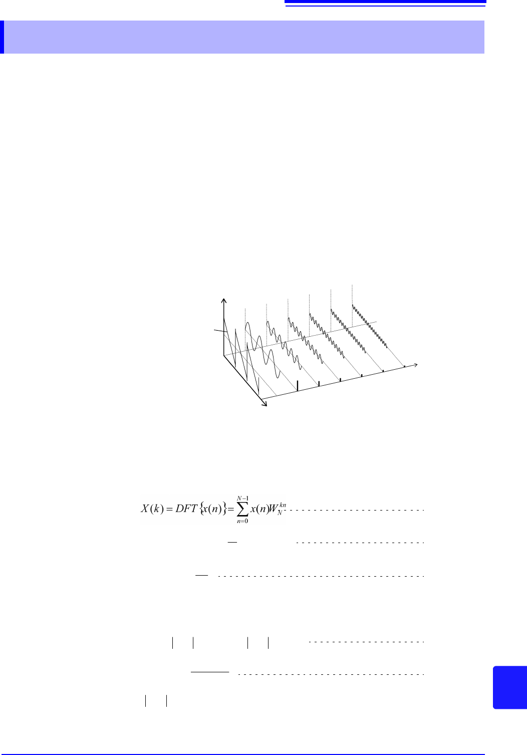
All signals are input to the instrument as a function of the time domain. This func-
tion can be considered as a combination of sine waves at various frequencies,
such as in the following diagram. The characteristics of a signal that may be diffi-
cult to analyze when viewed only as a waveform in the time domain can be eas-
ier to understand by transforming it into a spectrum (the frequency domain).
Discrete Fourier Transforms and Inverse FFT _______________________
For a discrete signal x(n), the DFT is X(k) and the number of Analysis points is N,
which relate as follows:
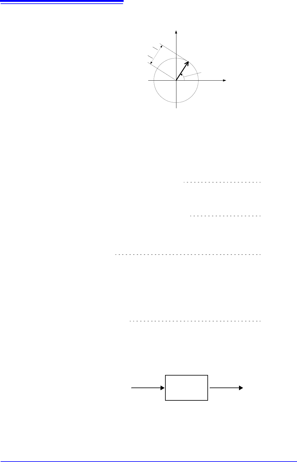
X(k) is typically a complex number, so expression (1) can be transformed again
and written as follows:
Appendix 4 FFT Definitions
Amplitude
Frequency
Time
Time-Domain
Waveform
(1)
kn
N
N
n
WkX
N
kXIDFTnx
1
0
)(
1
)()(
N
jW
N
2
exp
(2)
(3)
(4)
(5)
)()()(exp)()( kkFkjkFkF
)(Re
)(Im
tan)(
1
kX
kX
k
: Amplitude spectrum, : Phase spectrum
)(kF
)(k
Appendix 4 FFT Definitions
A14
Representing the above relationship on a complex flat surface produces the fol-
lowing figure.
Linear Time-Invariant Systems __________________________________
Consider a linear time-invariant (LTI) system y(n) that is a response to discrete
time-domain signal
x(n).
In such an LTI system, the following expression applies to any integer A
i
when
the response to x
i
(n) is y
i
(n) = L[x
i
(n)].
If the system function of an LTI system is h(n), the input/output relationship can
be obtained by the next expression.
Therefore, when a unit impulse (n) (which is 1 when n = 0, and 0 when n 0) is
applied to x(n), the input/output relationship is:
This means that when the input signal is given as a unit impulse, the output is
the LTI system characteristic itself.
The response waveform of a system to a unit impulse is called the impulse
response.
On the other hand, when the discrete Fourier transforms of x(n), y(n) and h(n) are
X(k), Y(k) and H(k), respectively, expression (7) gives the following:
H(k) is also called the transfer function, calculated from X(k) and Y(k). Also, the
inverse discrete Fourier transform function of H(k) is the unit impulse response
h(n) of the LTI system. The impulse response and transfer function of this instru-
ment are calculated using the relationships of expression (9).
)(kF
)(k
)
(
k
F
実数部
虚数部
Imaginary component
Real component
)()()]()([
22112211
nyAnyAnxAnxAL
(6)
(7)
mm
mxmnhmnxnhny )()()()()(
0
(8)
)()( nhny
(9)
)()()( kHkXkY
Input
(Analysis channel 1)
Output
(Analysis channel 2)
x(n)
X(k)
y(n)
Y(k)
h(n)
H(k)
LTI System
Appendix 4 FFT Definitions
A15
Appendix
Number of Analysis Points_______________________________________
The FFT functions of this instrument can perform frequency analysis of time-
domain waveforms consisting of 1000, 2000, 5000, or 10,000 points. However,
when the following conditions are satisfied, previously analyzed data can be
reanalyzed with a different number of analysis points.
A. When measurements are made with the averaging function disabled (Off)
B. When measurements are made with the averaging function enabled for time-
domain averaging (simple or exponential).
When the number of analysis points at measurement time is N
1
and the number
of analysis points is changed to N
2
after measurement, the instrument performs
as follows.
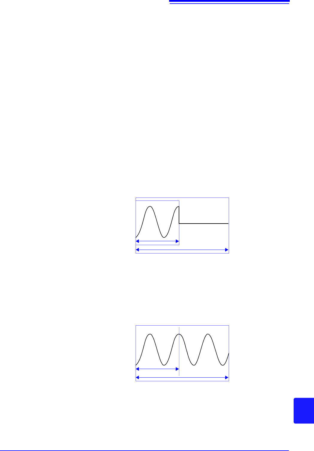
(1) When N
1
< N
2
• Because not enough data has been collected, zero is inserted for time after
the end of the measured waveform.
• The window function applies only to the N
1
segment.
• Frequency resolution is increased. For example, if N
1
= 1000 and N
2
= 2000,
frequency resolution is doubled.
• The average energy of the time-domain waveform is reduced, so the ampli-
tude of the linear spectrum is also reduced.
(2) When N
1
> N
2
• The specified (N
2
) segment is extracted from the head of the (N
1
) data.
• The window function applies only to the N
2
segment.
• Frequency resolution is decreased. For example, if N
1
= 2000 and N
2
= 1000,
frequency resolution is halved.
• The average energy of the time-domain waveform is unchanged, so the
amplitude of the linear spectrum is not significantly affected.
N
1
N
2
N
1
N
2