MR8740、MR8741_user_manual_eng_20191016H.pdf - 第411页
Appendix 4 FFT Definitions A 15 Appendix Number of Analysis Point s __ _____________________ ________________ The FFT functions of this instrument ca n perform fre quency analysis of time- domain wavefo rms consisting of…
Appendix 4 FFT Definitions
A14
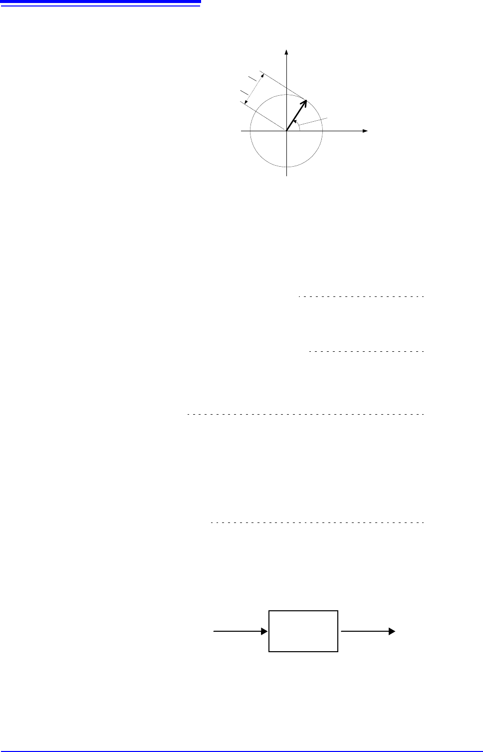
Representing the above relationship on a complex flat surface produces the fol-
lowing figure.
Linear Time-Invariant Systems __________________________________
Consider a linear time-invariant (LTI) system y(n) that is a response to discrete
time-domain signal
x(n).
In such an LTI system, the following expression applies to any integer A
i
when
the response to x
i
(n) is y
i
(n) = L[x
i
(n)].
If the system function of an LTI system is h(n), the input/output relationship can
be obtained by the next expression.
Therefore, when a unit impulse (n) (which is 1 when n = 0, and 0 when n 0) is
applied to x(n), the input/output relationship is:
This means that when the input signal is given as a unit impulse, the output is
the LTI system characteristic itself.
The response waveform of a system to a unit impulse is called the impulse
response.
On the other hand, when the discrete Fourier transforms of x(n), y(n) and h(n) are
X(k), Y(k) and H(k), respectively, expression (7) gives the following:
H(k) is also called the transfer function, calculated from X(k) and Y(k). Also, the
inverse discrete Fourier transform function of H(k) is the unit impulse response
h(n) of the LTI system. The impulse response and transfer function of this instru-
ment are calculated using the relationships of expression (9).
)(kF
)(k
)
(
k
F
実数部
虚数部
Imaginary component
Real component
)()()]()([
22112211
nyAnyAnxAnxAL
(6)
(7)
mm
mxmnhmnxnhny )()()()()(
0
(8)
)()( nhny
(9)
)()()( kHkXkY
Input
(Analysis channel 1)
Output
(Analysis channel 2)
x(n)
X(k)
y(n)
Y(k)
h(n)
H(k)
LTI System
Appendix 4 FFT Definitions
A15
Appendix
Number of Analysis Points_______________________________________
The FFT functions of this instrument can perform frequency analysis of time-
domain waveforms consisting of 1000, 2000, 5000, or 10,000 points. However,
when the following conditions are satisfied, previously analyzed data can be
reanalyzed with a different number of analysis points.
A. When measurements are made with the averaging function disabled (Off)
B. When measurements are made with the averaging function enabled for time-
domain averaging (simple or exponential).
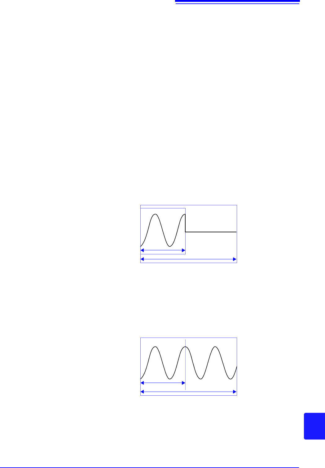
When the number of analysis points at measurement time is N
1
and the number
of analysis points is changed to N
2
after measurement, the instrument performs
as follows.
(1) When N
1
< N
2
• Because not enough data has been collected, zero is inserted for time after
the end of the measured waveform.
• The window function applies only to the N
1
segment.
• Frequency resolution is increased. For example, if N
1
= 1000 and N
2
= 2000,
frequency resolution is doubled.
• The average energy of the time-domain waveform is reduced, so the ampli-
tude of the linear spectrum is also reduced.
(2) When N
1
> N
2
• The specified (N
2
) segment is extracted from the head of the (N
1
) data.
• The window function applies only to the N
2
segment.
• Frequency resolution is decreased. For example, if N
1
= 2000 and N
2
= 1000,
frequency resolution is halved.
• The average energy of the time-domain waveform is unchanged, so the
amplitude of the linear spectrum is not significantly affected.
N
1
N
2
N
1
N
2
Appendix 4 FFT Definitions
A16
Aliasing ______________________________________________________
When the frequency of a signal to be measured is higher than the sampling rate,
the observed frequency is lower than that of the actual signal, with certain fre-
quency limitations. This phenomena occurs when sampling occurs at a lower fre-
quency than that defined by the Nyquist-Shannon sampling theorem, and is
called aliasing.
If the highest frequency component of the input signal is f
max
and the sampling
frequency is f
s
, the following expression must be satisfied:
Therefore, if the input includes a frequency component higher than f
s
/2, it is
observed as a lower frequency (alias) that does not really exist.
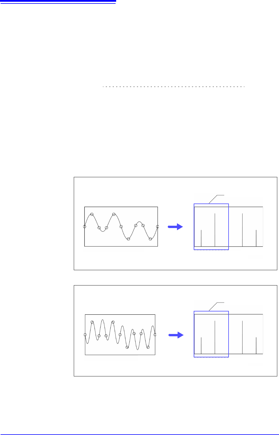
The following diagrams show the results of spectrum analysis of composite
waveforms having components of 1 kHz and 3 kHz, and of 1 kHz and 7 kHz.
If sampling frequency f
s
is 10 kHz, the spectral component of an input frequency
above 5 kHz (in this case, 7 kHz) is observed as an alias at 5 kHz or below.
In this example the difference between the 3 and 7 kHz components is indiscern-
ible.
max
2 ff
s
(10)
Composite waveform of 1 kHz and 3 kHz components sampled at 10 kHz
Time
Portion Displayed on
Screen
Spectrum
1357
Frequency
[kHz]
Composite waveform of 1 kHz and 7 kHz components sampled at 10 kHz
Time
Spectrum
Frequency
[kHz]
1357
Portion Displayed on
Screen