MR8740、MR8741_user_manual_eng_20191016H.pdf - 第265页
12.3 Setting FFT Analysis Conditio ns 253 11 Chapter 12 FFT Function 12 When performing FFT analysis of data measur ed using the memory function, the mea surement data can be thinned bef ore calculation. If the sampling …

12.3 Setting FFT Analysis Conditions
252
Relationship Between Frequency Range, Resolution and Number of
Analysis Points
Range
[Hz]
Sampling
frequency
[Hz]
Timebase
[/div]
(MEM)
Sampling
period
Number of FFT Analysis Points
1,000 2,000 5,000 10,000
Resolu-
tion [Hz]
Acquisi-
tion
interval
Resolu-
tion [Hz]
Acquisi-
tion
interval
Resolu-
tion [Hz]
Acquisi-
tion
interval
Resolu-
tion [Hz]
Acquisi-
tion
interval
8 M *
1
20 M 5 s 50 ns 20 k 50 s 10 k 100 s 4 k 250 s 2 k 500 s
4 M *
1
10 M 10 s 100 ns 10 k 100 s5 k200 s 2 k 500 s1 k1 ms
2 M *
1
5 M 20 s 200 ns 5 k 200 s 2.5 k 400 s 1 k 1 ms 500 2 ms
800 k *
1
2 M 50 s 500 ns 2 k 500 s 1 k 1 ms 400 2.5 ms 200 5 ms
400 k *
1
1 M 100 s1 s 1 k 1 ms 500 2 ms 200 5 ms 100 10 ms
200 k *
1
500 k 200 s2 s 500 2 ms 250 4 ms 100 10 ms 50 20 ms
80 k *
1
200 k 500 s5 s 200 5 ms 100 10 ms 40 25 ms 20 50 ms
40 k
100 k 1 ms 10
s 100 10 ms 50 20 ms 20 50 ms 10 100 ms
20 k
50 k 2 ms 20
s 50 20 ms 25 50 ms 10 100 ms 5 200 ms
8 k
20 k 5 ms 50
s 20 50 ms 10 100 ms 4 250 ms 2 500 ms
4 k
10 k 10 ms 100
s 10 100 ms 5 200 ms 2 500 ms 1 1 s
2 k
5 k 20 ms 200 s 5 200 ms 2.5 400 ms 1 250 ms 500 m 2 s
800
2 k 50 ms 500 s 2 500 ms 1 1 s 400 m 2.5 s 200 m 5 s
400
1 k 100 ms 1 ms 1 1 s 500 m 2 s 200 m 5 s 100 m 10 s
200
500 200 ms 2 ms 500 m 2 s 250 m 4 s 100 m 10 s 50 m 20 s
80
200 500 ms 5 ms 200 m 5 s 100 m 10 s 40 m 25 s 20 m 50 s
40
100 1 s 10 ms 100 m 10 s 50 m 20 s 20 m 50 s 10 m 100 s
20
50 2 s 20 ms 50 m 20 s 25 m 40 s 10 m 100 s 5 m 200 s
8 *
2
20 5 s 50 ms 20 m 50 s 10 m 100 s 4 m 250 s 2 m 500s
4 *
2
10 10 s 100 ms 10 m 100 s 5 m 200s 2 m 500 s 1 m 1 ks
1.33 *
2
3.33 30 s 300 ms 3.33 m 300 s 1.66 m 600s 666 1.5 ks 333 3 ks
800 m *
2
2 50 s 500 ms 2 m 500 s 1 m 1 ks 400 2.5 ks 200 5 ks
667 m *
2
1.67 60 s 600 ms 1.66 m 600 s 833 1.2 ks 333 3 ks 166 6 ks
400 m *
2
1 100 s 1 s 1 m 1 ks 500 2 ks 200 5 ks 100 10 ks
333 m *
2
833 m 120 s 1.2 s 833 1.2 ks 416 2.4 ks 166 6 ks 83.3 12 ks
133 m *
2
333 m 300 s 3 s 333 3 ks 166 6 ks 66.6 15 ks 33.3 30 ks
The cut-off frequency of the anti-aliasing filter is the same as the frequency range.
*1. The anti-aliasing filter is turned off.
*2. Cut-off frequency is 20 Hz.
12.3 Setting FFT Analysis Conditions
253
11
Chapter 12 FFT Function
12
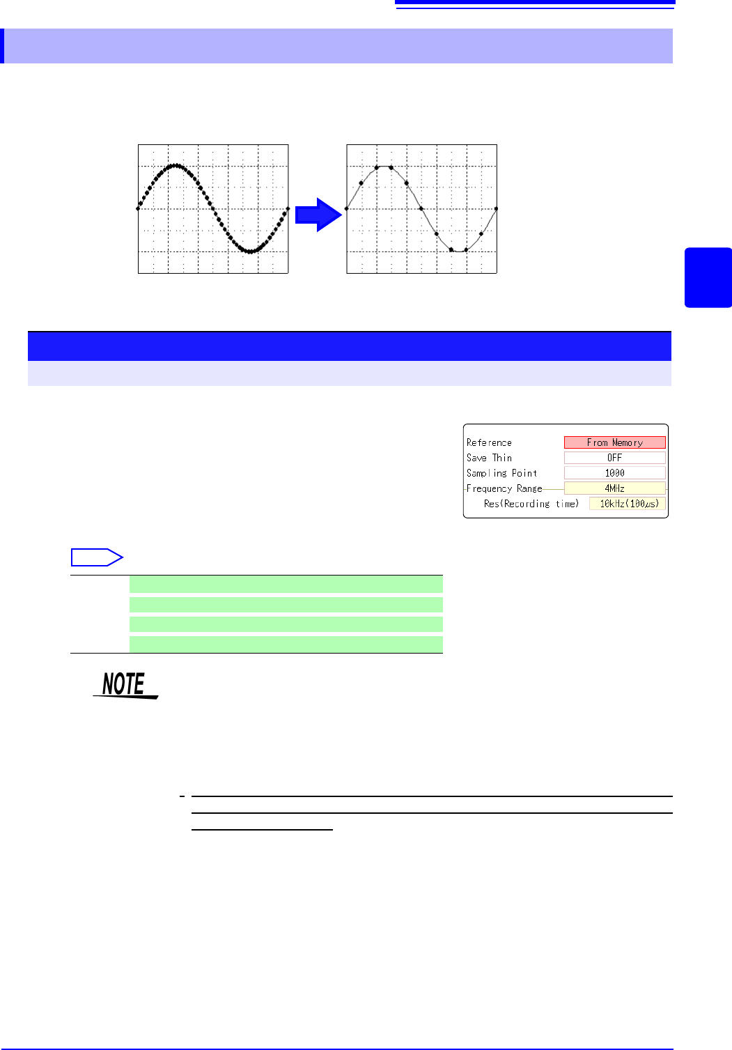
When performing FFT analysis of data measured using the memory function, the measurement
data can be thinned before calculation. If the sampling frequency is too high and the expected
results are not obtained, thin the data before calculation to increase the frequency resolution.
12.3.4 Thinning Out and Calculating Data
Original waveform Thinned waveform
1
Select the reference data.
Move the flashing cursor to the [Reference] item, and select
[From Memory].
2
Select the thinning amount.
Move the flashing cursor to the [Save Thin] item.
Select
Off Do not thin out.. (default setting)
1/10
Skip every 10 data points.
1/100
Skip every 100 data points.
1/1000
Skip every 1000 data points.
Procedure
To open the screen: Right-click and select [STATUS] [Status] sheet
1
2
• The [Save Thin] setting can only be set when the [Reference] is set to [From
Memory].
• The range that can be set for thinning changes depending on the time axis
range measured by the memory function.
• The frequency range is automatically determined. This setting cannot be
changed.
•
When thinning, aliasing occurs and waveforms that did not originally exist may
be observed. Make settings after sufficient consideration of the frequencies
included in waveforms.
12.3 Setting FFT Analysis Conditions
254
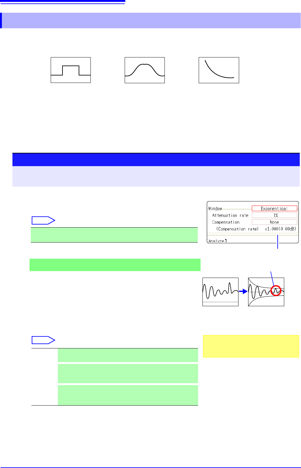
The window function defines the segment of the input signal to be analyzed.
Use the window function to minimize leakage errors. There are three general types of window functions:
The non-rectangular window functions generally produce lower-level analysis results. By applying attenu-
ation correction, the attenuation introduced by the non-rectangular window functions can be corrected to
bring analysis results back to similar levels.
12.3.5 Setting the Window Function
• Rectangular Window
• Hann window
• Hamming window
• Blackman window
• Blackman-Harris window
• Flat top window
• Exponential window
1
Select the window function.
Move the flashing cursor to the [Window] item.
Select
See: "Window Function" (p.A21)
2
If [Exponential] is the selected type
Set the attenuation coefficient (percentage).
Move the flashing cursor to the [Attenuation rate] item.
Set the attenuation coefficient as a percentage.
3
Set attenuation correction.
Move the flashing cursor to the [Compensation] item.
Select
Rectangular (default setting), Hanning, Hamming, Blackman, Black-
man Harris, Flat-top, Exponential
None Attenuated window function values are not corrected.
(default setting)
Power
The window function multiplies the power levels of the time-do-
main waveform so that output levels are comparable to those
of a rectangular window.
Average
The window function multiplies the average value of the time-
domain waveform so that output levels are comparable to
those of a rectangular window.
Procedure
To open the screen: Right-click and select [STATUS] [Status] sheet
See: To set from the Waveform screen (p.265)
Correction value
For the rectangular window function:
The correction value is always 1 (0 dB).
When the attenuation rate is 10%
10%
100%
Noise is suppressed in the attenuated wave-
form.
2
1
3