IPC-TM-650 EN 2022 试验方法.pdf - 第326页
5.3.2 An idealized TMA curve has a linear section below the transition (expansion below T g ) and a linear section above the transition (expansion above T g ). These linear sections are used in calculating the T g and CT…
5.2.1.2
Apply the Load
Method A
Mount
the specimen on the stage of the TMA
and apply load at 5 g (see 6.5 for an explanation of load cri-
teria). Enclose the specimen and probe in the environmental
chamber.
Method
B
Mount
the specimen in the clamps of the film fix-
ture according to the manufacturer’s instructions and apply 2
g tension force (see 6.5 for an explanation of the load criteria).
Enclose the specimen and probe in the environmental cham-
ber.
5.2.1.3
Provide
an inert gas purge (helium or nitrogen) at a
rate of 30 ml/min to 150 ml/min to the environmental cham-
ber. Temperature calibration of the TMA must be performed
under the same gas conditions.
5.2.1.4
Measure
the inital specimen thickness (Method A) or
length (Method B) prior to each heat cycle (L
O
).
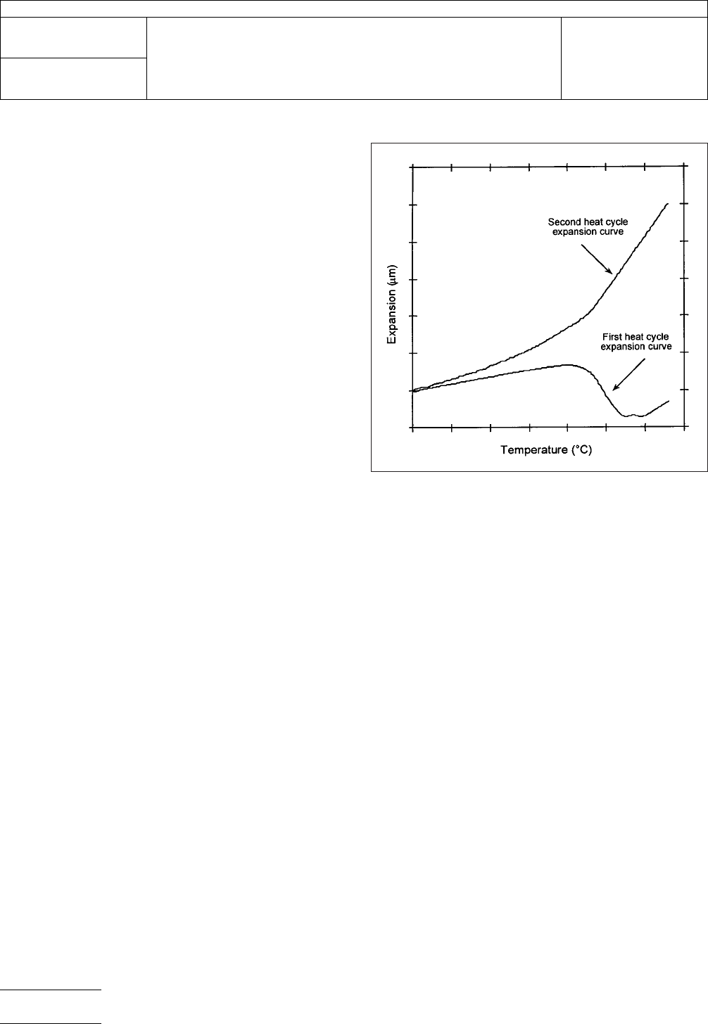
5.2.2
Many
specimens have built in thermal stresses from
the curing step, which relaxes during the specimen heating
during a TMA test. This relaxation results in TMA scans, which
make determination of T
g
and
CTE impossible (see Figure 1).
Two heat cycles are required to obtain valid T
g
and
CTE val-
ues.
5.2.3
Running the TMA Temperature Scan
5.2.3.1
Initial
Temperature (T
initial
)
a.
For specimens with T
g
below
or near room temperature,
start the scan at least 20°C below the anticipated transi-
tion. This may require a TMA with refrigeration control of
the environmental chamber.
b. For specimens with T
g
greater
than room temperature,
start the scan at 30°C.
5.2.3.2
Temperature Rate
Depending
on sample prepa-
ration, two heating cycles may be required to obtain accurate
T
g
and
CTE above T
g
.
If the sample shows unexpected
shrinkage above T
g
(see
Figure 1), the two heat test method
is required. If the sample does not show anomalous behavior,
only one heat cycle (the second heat cycle at 5°C/min) is
required.
a. First heat: The first heat cycle of the specimen shall be run
at 10°C/min.
b. Second heat (reportable data heat cycle): The second
heat cycle of the specimen shall be run at 5°C/min.
5.2.3.3
Temperature Excursion
a.
First heat: Continue heating the specimen to a tempera-
ture 20°C greater than the anticipated T
g
or
until the
anomalous thermal relaxation has stopped. See Figure 1
for an example of anomalous first heat behavior. Hold the
specimen at this temperature for a minimum of five min-
utes. Avoid holding the sample at this temperature for too
long; sample degradation might occur. Cool the specimen
to the initial temperature under temperature control at
5°C/min to 10°C/min. This should prevent reestablishment
of thermal stresses.
b. Second heat (reportable data heat cycle): The second
heat cycle of the specimen shall continue to 310°C (to
ensure good data at 300°C).
5.3
Evaluation
5.3.1
The
TMA expansion curve should resemble the plot
shown in Figure 2.
IPC-24245-1
Figure
1 TMA Expansion Curves: First Heat Cycle and
Second Heat Cycle
IPC-TM-650
Number
2.4.24.5
Subject
Glass
Transition Temperature and Thermal Expansion of
Materials Used in High Density Interconnection (HDI) and
Microvias - TMA Method
Date
11/98
Revision
P
age2of5
电子技术应用 www.ChinaAET.com
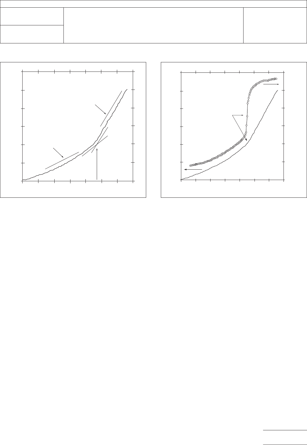
5.3.2
An
idealized TMA curve has a linear section below the
transition (expansion below T
g
)
and a linear section above the
transition (expansion above T
g
).
These linear sections are
used in calculating the T
g
and
CTE of the material.
With real samples, these ‘‘linear’’ sections are often curved so
the standard CTE calculation (see 5.4.2) is the average CTE
between the defined points (A-B and C-D in Figure 2). The
instantaneous CTE provides CTE as a function of temperature
and avoids this averaging effect (see Figure 3).
5.3.3
From
the TMA plot, pick four temperatures and obtain
the specimen thicknesses at these temperatures:
T
A
–
at least 10°C above T
initial
(to
ensure thermal equilibrium)
and no higher than 25°C above T
initial
T
B
–
on the linear portion of the graph below the T
g
T
C
–
on the linear portion of the graph above T
g
T
D
–
300°C
Preferred temperatures for HDIS materials:
T
initial
=
30°C
T
A
=
40°C
T
B
=
material dependent - below the T
g
T
C
=
material dependent - above T
g
T
D
=
300°C
5.3.4
Examine
all specimens after the test to look for signs
of excessive loads, distortions, tears, and other defects. If any
defects or sample irregularities are found, discard the sample
and the data, rerun another specimen, or pick a different
method for determining T
g
and
CTE.
5.4
Calculations
5.4.1 Glass Transition Temperature – T
g
Construct
a
tangent line to the curve above and below the transition in the
curve. The temperature where these tangents intersect is the
TMA determined T
g
for
the material. If the tangent method fails
to provide an adequate T
g
,
the instantaneous CTE can be
calculated (see 5.4.3) and the midpoint of the step change in
CTE may be taken as T
g
(see
Figure 3). For consistency, it is
recommended that the TMA computer analysis software be
used for this calculation (see Figure 2).
5.4.2
Mean Coefficient of Thermal Expansion – CTE
The
mean CTE shall be calculated over the specified regions
and recorded in units of ppm/°C. For consistency it is recom-
mended that the TMA computer analysis software be used for
this calculation.
IPC-24245-2
Figure
2 TMA Expansion Curve
Slope in this region:
CTE abo
ve T
g
Slope in this region:
CTE belo
w T
g
T
g
T
emperature (˚C)
Expansion (µm)
A
B
C
D
IPC-24245-3
Figure
3 TMA Expansion Curve and Instantaneous CTE
Curve
Instantaneous CTE Cur
ve
T
g
60
50
40
30
20
10
0
Expansion Cur
ve
0
40
80
120
160
200
240
Temperature (˚C)
Expansion (µm)
CTE (ppm)
IPC-TM-650
Number
2.4.24.5
Subject
Glass
Transition Temperature and Thermal Expansion of
Materials Used in High Density Interconnection (HDI) and
Microvias - TMA Method
Date
11/98
Revision
P
age3of5
电子技术应用 www.ChinaAET.com

a.
CTE below glass transition:
α
(B–A
)
=
(L
B
–L
A
)10
6
L
o
(T
B
–T
A
)
For
most materials, this will be in the range of 7 ppm to 50
ppm (reinforced) or 30 ppm to 150 ppm (unreinforced).
b. CTE above glass transition:
α
(D–C
)
=
(L
D
–L
C
)10
6
L
o
(T
D
–T
C
)
For
most materials, this will be in the range of 50 ppm to 100
ppm (reinforced) or 150 ppm to 500 ppm (unreinforced). Any
reinforced materials, where the reinforcement has a negative
CTE, will shrink rather than expand when heated above T
g
of
the
resin.
Where:
T
A
=
Temperature at point A in Figure 2
T
B
=
Temperature at point B in Figure 2
T
C
=
Temperature at point C in Figure 2
T
D
=
Temperature at point D in Figure 2
L
0
=
Initial Length or thickness
L
A
=
Length or thickness at point A in Figure 2
L
B
=
Length or thickness at point B in Figure 2
L
C
=
Length or thickness at point C in Figure 2
L
D
=
Length or thickness at point D in Figure 2
5.4.3
Instantaneous Coefficient of Thermal Expansion
Curve (Optional)
The
instantaneous CTE expansion curve
is the slope of the TMA expansion curve plotted as a function
of temperature. Figure 3 shows a combined expansion curve
and its resulting instantaneous CTE curve.
Instantaneous CTE (α
Ti
)
is calculated at each temperature (T
i
)
from
the slope of the TMA expansion curve (dL
i
/dT)
at that
temperature:
α
Ti
=
1
L
o
(
dL
i
dT
)
dL/dT
is determined at each temperature (T
i
)
from the L vs. T
curve by:
(
dL
i
dT
)
=
(L
i+1
− L
i
)
(T
i + 1
− T
i
)
This
calculation can be done in a spreadsheet that contains
the L vs. T data. Some TMA computer analysis software per-
forms this calculation for you. For an example of plot αη
Ti
vs
temperature,
see Figure 3.
5.4.4
Percent Thermal Expansion (PTE) (Optional)
The
total
percent of thermal expansion is calculated as follows:
Percent TE =
(T
D
–T
A
)
L
o
*
100
For consistency, it is recommended that the TMA computer
analysis software be used for this calculation.
5.5
Report
5.5.1
Report
the glass transition temperature of each speci-
men, rounding to the nearest whole number.
5.5.2
Report
the CTE in ppm/°C above and below T
g
and
the
temperature ranges over which the thermal expansion
was determined. For Method B, report x and y CTE values.
5.5.3 Optionally
report the PTE in percent and the tempera-
ture ranges over which the thermal expansion was deter-
mined.
5.6 Plot
5.6.1
Plot
the expansion (µm) vs. temperature (°C) for the
specimen. If using computer based analysis, include the T
g
and
CTE measurement start points and computer generated
lines (see Figure 2).
5.6.2
Optionally
plot the instantaneous CTE (µm/°C) vs.
temperature (°C) for the specimen (see Figure 3).
5.6.3
Optionally
plot the percent expansion vs. temperature
(°C) for the specimen. If using computer-based analysis,
include the PTE measurement start points on the plot.
6.0
Notes
6.1
Calibration
of the TMA must be carried out according to
the manufacturer’s instructions for both probe expansion and
specimen temperature.
IPC-TM-650
Number
2.4.24.5
Subject
Glass
Transition Temperature and Thermal Expansion of
Materials Used in High Density Interconnection (HDI) and
Microvias - TMA Method
Date
11/98
Revision
P
age4of5
电子技术应用 www.ChinaAET.com