IPC-TM-650 EN 2022 试验方法.pdf - 第534页

operation is specified in Equation 5-2. I_R j = RB j − RB j − 1 t j − t j − 1 I_T j = TB j − TB j − 1 t j − t j − 1 [5-2] 5.2.2.4 RIE Results The reference structure, RIE reference ,i s the square root of the square of t…

These are the TDR waveforms used in the RIE loss calcula-

tion.

It is recommended to be positioned within 80% of the vertical

screen scale in reference to the representative waveform. The

signal on the screen must have a resolution of at least 5% of

the measured signal.

Figure 5-3 specifies two time regions. T0 and T1. The sum of

T0 and T1 represents the time range for the captured wave-

form. Figure 5-3 specifies the point between T0 and T1 which

corresponds to the point where the probe contacts the

printed board, or where the rising edge would be if the probe

were disconnected from the sample. The TDR specification

for T0 and T1 is found in Table 5-1.

Each TDR waveform is averaged on the TDR instrument at

least 16 times. The time base and offset remain the same for

all measurements.

5.2.2 Measurement and Processing Two TDR wave-

forms are captured. One corresponds to a reference and the

second corresponds to the test line.

The measured waveforms require post-processing. TDR

waveform is processed as follows:

a) Filtering

b) Cubic spline fit

c) Using derivative to find impulse response

d) Calculating RIE loss ratio

5.2.2.1 Recursive Digital Filtering of Spline Data The

two TDR waveforms are filtered using the method prescribed

in Equation 5-1.

Let S

j,0

= A

for k = 1 to N

j,k

2,k +

i=1

(

i-1

⋅ S

i,k

)

Assign B

= S

j,N

[5-1]

Where:

N is the number of filtering iterations

is the j

point of the on of the acquired TDR waveforms

Sj,k is the j

point of the k

filtered waveform

j is an index for the waveform points

Bj is the j

point of the filtered waveform

The number of filter iterations depends on the number of

samples in the acquired TDR waveform and specified in Table

5-2.

5.2.2.2 Resampling with a Cubic Spline Fit The next

step is to resample the filtered TDR data to 10,000 points (J).

This is accomplished with a cubic spline fit.

5.2.2.3 Impulse Response The impulse response of the

reference and test specimen, respectively I_R

and I_T

is cal-

culated by taking the derivative of the respective resample

step waveforms RB

and TB

. One method to perform this

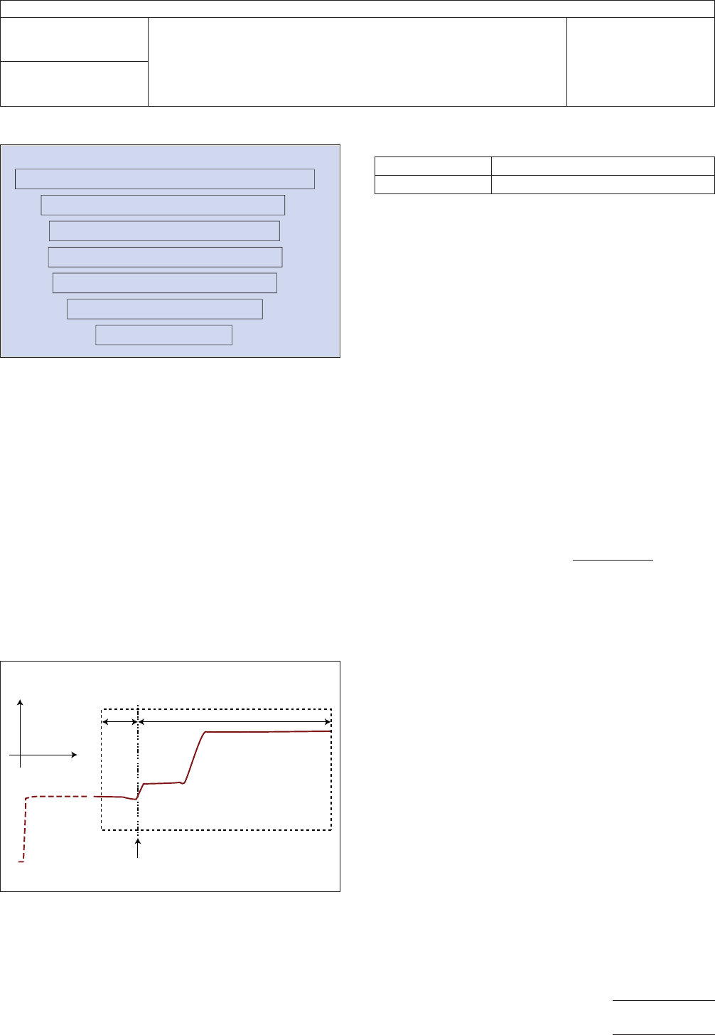
Figure 5-2 RIE Flowchart

RIE TDR PROCESS

Acquire TDR response for one reference and line under test

Averaging filter of re-sampled TDR waveforms

Cubic spline re-sampling of TDR waveforms

Perform Derivative of filtered TDR waveforms

Determine RIE loss from reference Sample

Determine RIE loss from test Sample

Determine RIE loss ratio

IPC-25512-5-3

Figure 5-3 Waveform Position on TDR Screen

Voltage

Time

Corresponds to probe launch

T0 T1

TDR Display Window for RIE

Table 5-1 RIE TDR Time Range Speciﬁcations

T0 50 ps (typical)

T1 At least twice the transit delay

IPC-TM-650

Number

2.5.5.12

Subject

Test Methods to Determine the Amount of Signal Loss on

Printed Boards

Date

07/12

Revision

Page 13 of 24

operation is specified in Equation 5-2.

I_R

− RB

j−1

− t

j−1

I_T

− TB

j−1

− t

j−1

[5-2]

5.2.2.4 RIE Results The reference structure, RIE

reference

,is

the square root of the square of the integral of the square of

the impulse response I_R, and can be calculated from J

samples as show in Equation 5-3. The test structure, RIE

test

is the square root of the square of the integral of the square

of the impulse response I_T, and is calculated from J samples

as show in Equations 5-3 and 5-4.

RIE

reference

√

j=1

I_R

− t

)

[5-3]

RIE

test

√

j=1

I_T

− t

)

[5-4]

The RIE loss in dB, RIE

loss_dB

, is calculated by dB ratio of the

RIE

test

to RIE

reference

as show in Equation 5-5.

RIE

loss_db

= 20 * log

(

RIE

test

RIE

reference

)

[5-5]

5.3 SPP Procedure Figure 5-4 summarizes the SPP mea-

surement extraction process.

5.3.1 Selecting Optimum SPP Transmission Lines SPP

utilizes measurements on two lines of different lengths such as

2.0 cm and 8.0 cm. The pair shall be designed to be identi-

cal in every way except for length. The SPP is used to extract

parameters such as α(f) β(f), Γ(f) and Z

(f) by utilizing the dif-

ference between the two specimen line lengths. Effects due to

the connectors, cables, probes, and oscilloscope circuitry can

be minimized using this method. Screening the two lines

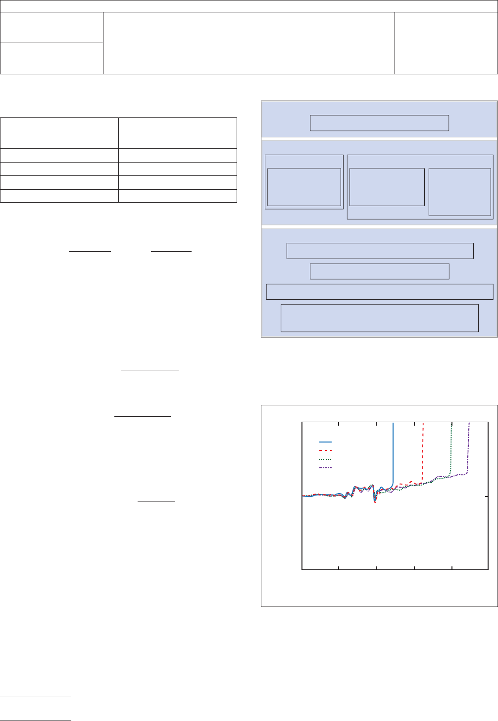
improves accuracy. Figure 5-5 illustrates lines of similar

design. Accuracy is improved when the slope and deviation

along the lengths of overlaid portions of the respective TDR

waveforms are coincident.

5.3.1.1 Additional SPP Step for Differential Lines There

are a few additional steps needed when analyzing differential

lines. The TDR screening still needs to be performed first. In

Table 5-2 Filter iterations, N, vs.

number of points, n, in TDR capture

Number of Points

in TDR capture (n)

Number of

Filtering Iterations

(N in Equation 5-1)

0>n≥750 1

750>n≥1500 2

1500 > n ≥3000 6

> n >3000 21

Figure 5-4 SPP Flowchart

TDR

Select best candidates for line pairs

Low Freq

TDT

disc

Determine

1MHzε

and Tan δ

(LCR meter)

Determine

Capacitance/unit

length (LCR meter)

Determine

Resistance/unit

length ρ and

(LCR meter)

Lines

Acquire Impulse response for 2 lines of 2 lengths

Window and filter Impulse response

FFT to get Propagation Constant Γ (Attenuation and Phase)

Use itrative matching of Γ, Att, and low freq

parameters to determine tline modeling parameters

IPC-25512-5-5

Figure 5-5 Example of Similar TDR Responses for

Different Lengths of Lines

0.3

0.2

0.25

1.5 2.5

Time (nsec)

Voltage (V)

3.52

1=2 cm

1=5 cm

1=8 cm

1=9.8 cm

IPC-TM-650

Number

2.5.5.12

Subject

Test Methods to Determine the Amount of Signal Loss on

Printed Boards

Date

07/12

Revision

Page 14 of 24

this case, the screening has to be done for odd-mode, with

TDR pulse polarity of + -, and even-mode, + +. It is also rec-

ommended to perform TDR for +0 and 0+ single mode to see

how close to each other the two lines’ characteristics are.

5.3.2 Measuring Frequency Relative Permittivity with

SPP

The capacitance shall be measured at 1 MHz with an

LCR meter for several lengths of lines. Such measurements

are generally made at a low enough frequency such as 1 MHz

so that the reactance associated with the lead inductance is

negligible. In a subsequent step line resistance measurements

usinga4wireKelvin method are also made. The measure-

ments determine the resistance per unit length and the

capacitance per unit length. By taking the difference between

results at two lengths and dividing by the difference in lengths,

the effect of parasitic end load is eliminated. The LCR meter

shall be also used to measure the capacitance between the

layers of the large circular disc designated for dielectric per-

mittivity determination.

Relative permittivity, ε

, is calculated with Equation 5-6 using

the known area, A, of the test specimen disc, the distance

between the layers h, and the capacitance, C, as measured

with the LCR at 1 MHz. The value for ‘‘h’’ may be determined

by cross-sectioning analysis.

[5-6]

5.3.3 Measuring Low Frequency Copper Resistivity, ρ,

with SPP

The resistivity (ρ) per unit length of the signal line

conductor is determined with Equation 5-7. R

is the resis-

tance measured usinga4wireKelvin method for the long line

of length l

. R

is the resistance measured usinga4wireKel-

vin method for the short line of length l

ρ=

− R

− l

[5-7]

A is the cross-section area (equal to the conductor width mul-

tiplied by the conductor thickness).

5.3.4 SPP Low Frequency Permittivity It should be

noted that the two ground planes that are above and below

the signal of interest are always shorted together, in the trans-

mission line region and in the parallel plate disc area. The disc

that is used should have a diameter that is 100x the height, h

to, the nearest ground in order to be able to calculate ε

directly from (1) without any fringe capacitance consideration.

The typical diameter of the disc is 12.7 mm [0.5 in]. It is use-

ful to have a dummy structure that is nearby the disc that has

only the via connection between the surface pad and the disc

and the small lateral line extension. Typical configuration was

shown in 3.3.4.2. The capacitance of this parasitic structure is

subtracted from the total disc C so that the end effects are not

included in the result for ε

Finally, the dielectric loss, tanδ, is also measured for the large

disc using the same LCR meter in the range of 10 KHz to

1 MHz.

The line capacitance per unit length, together with the cross

sectional dimensions can also be used for determining the

dielectric constant at 1 MHz. The procedure is to calculate the

capacitance with a 2D field solver for an assumed dielectric

constant. Iteration is used on this assumed value until the

agreement is obtained between measured and calculated C.

The implicit assumption here is that the lines are uniform and

that the cross section is well known along the length. Both

these assumptions have limitations and this is why the extrac-

tion based on line C is not as accurate. On the other hand, the

composition of glass fiber and dielectric resin might differ in

the disc area from the line area which could introduce errors

in the extracted ε

at 1 MHz.

5.3.5 SPP TDT Measurement TDT measurements are

also made with several lines, but especially with the 2 cm

[0.787 in] and 8 cm [3.15 in] lines of interest. In addition, it is

useful to measure a very short line of ‘‘zero length,’’ (e.g., 0.25

- 0.45 mm [0.0098 - 0.0177 in]) in order to obtain the band-

width of the time-domain set-up and for use as a reference for

delay extraction. The TDT measurement monitors the propa-

gation delay at 50% of the signal swing, the propagated rise

time between 10% and 90% levels. By taking the difference in

delays for the two lines and dividing by the difference in

lengths, one obtains the line propagation delay per unit length,

τ, without the effect of probes, pads, and via discontinuities.

The assumption is that these features are of similar character-

istics for the two lines. The propagated risetime through the

‘‘zero length’’ line indicates the bandwidth for the setup based

on the simplified formula for the upper 3 dB frequency given

in Equation 5-8.

, =

0.35

[5-8]

The correlation of propagation delay and rise time shape with

simulation can provide a very useful validation of the broad-

band model that is being created using this method.

Examples are given in Figure 5-6.

IPC-TM-650

Number

2.5.5.12

Subject

Test Methods to Determine the Amount of Signal Loss on

Printed Boards

Date

07/12

Revision

Page 15 of 24