semi合集-English.pdf - 第102页

SEMI E10-0304 E © SEMI 1986, 2004 16 A2-2.5 In this equation z critical comes from the critical values of the st andard normal distri bution (for 90% significance, z critical = 1.282, for 95% significance, z critical = 1…

SEMI E10-0304

APPENDIX 2

RELIABILITY GROWTH OR DEGRADATION MODELS

NOTICE: This appendix was approved as an official part of SEMI E10 by full letter ballot procedure. It offers detailed

information related to Section 8.

A2-1 Introduction

A2-1.1 E-MTBF

may be substituted for MTBF

in all

calculations in this section.

A2-1.2 If the times between failures (known as

“interarrival times”) of a repairable system or piece of

equipment are independent random times sampled from

the same exponential distribution, then the (theoretical)

rate of occurrence of failures (“ROCOF”) is a constant

λ and the MTBF

is just 1/λ. This situation is known in

the reliability literature as a homogeneous poisson

process (HPP). An HPP assumption underlies the

definition of MTBF

given in Section 6, and the

confidence limit factors described in Section 7 and

Appendix 1. These concepts are described in detail in

Ascher and Feingold [1] and Tobias and Trindade [2].

A2-1.3 If reliability is either improving or degrading

with time, then the ROCOF is no longer a constant and

a MTBF

calculation will be misleading.

A2-1.4 This appendix contains a simple test for trend

that may be applied if a time-varying ROCOF is

suspected, as well as a description of a well known and

powerful model that may be used when reliability

improvement trends are evident in the equipment

failure time data.

A2-2 Testing for Trends

A2-2.1 A non-parametric reverse arrangement test

(RAT) devised by Kendall [3] and further developed

into a table by Mann [4] will be described. Begin by

writing the interarrival times in the order they occurred.

For a period with r failures, these might be X

, X

, …,

. Starting from left to right, define a reversal as any

instance in which a lesser value occurs before any

subsequent greater value in the sequence. In other

words, any time we have X

< X

and i < j, we count it

as a reversal. For example, suppose a piece of

equipment has r = 4 failures at 30, 160, 220, and 360

hours of productive time. The interarrival times are 30,

130, 60, and 140. The total number of reversals is 3 + 1

+ 1 = 5.

A2-2.2 A larger than expected number of reversals

indicates an improving trend; a smaller number of

reversals than expected indicates a degradation trend.

A2-2.3 For r up to 12, use Table A2-1 below (adapted

from [2]) to determine whether a given number of

reversals, R, is statistically significant at the 100 × (1 –

α) confidence level.

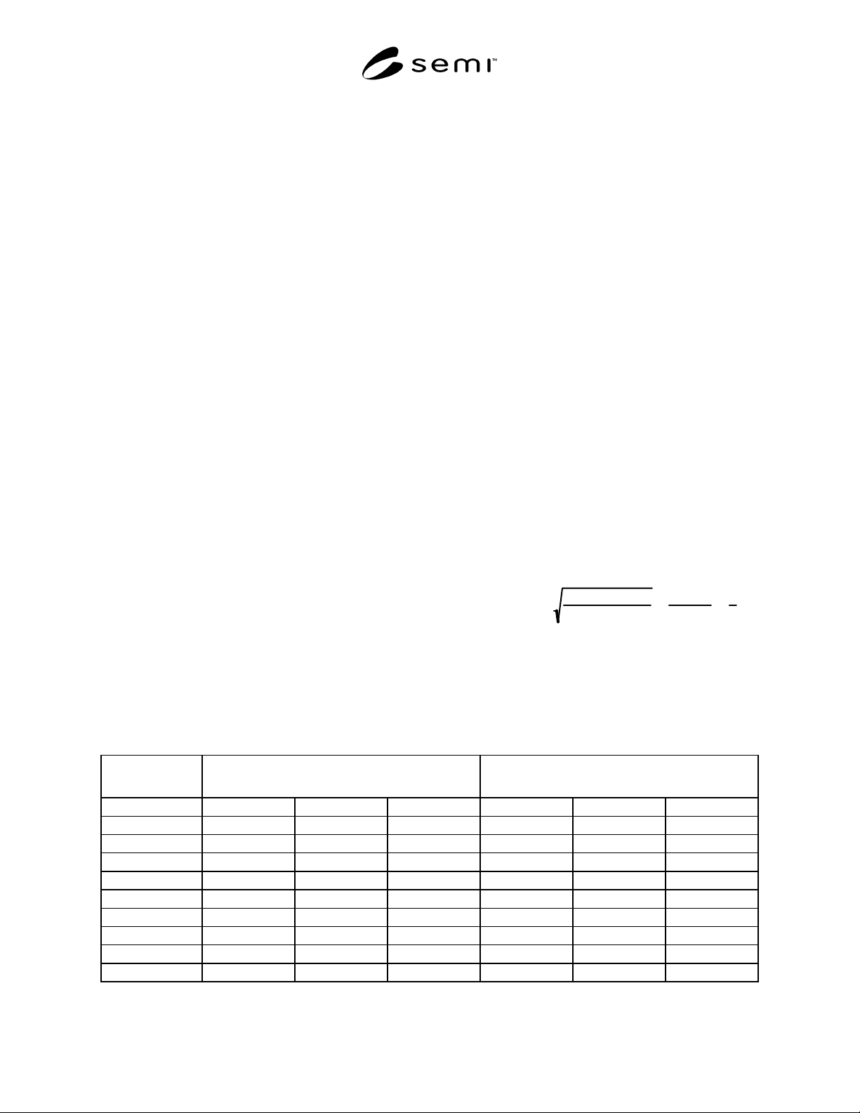
A2-2.4 For r greater than 12, approximate critical

values for the number of reversals (based on Kendall’s

normal approximation) can be calculated from:

(r; 1-

)

= z

critical

(2r

5)(r − 1)r

r(r

−

Table A2-1 Critical Values R

r;1-

the Number of Reversals for the Reverse Arrangement Test at a Given

Confidence Level

Sample Size Single-Sided Lower Critical Value (Too Few

Reversals Provide Evidence of Degradation)

Single-Sided Upper Critical Value (Too Many

Reversals Provide Evidence of Improvement)

r 99% 95% 90% 90% 95% 99%

4 0 0 6 6

5 0 1 1 9 9 10

6 1 2 3 12 13 14

7 2 4 5 16 17 19

8 4 6 8 20 22 24

9 6 9 11 25 27 30

10 9 12 14 31 33 36

11 12 16 18 37 39 43

12 16 20 23 43 46 50

SEMI E10-0304

A2-2.5 In this equation z

critical

comes from the critical

values of the standard normal distribution (for 90%

significance, z

critical

= 1.282, for 95% significance, z

critical

= 1.645, and for 99% significance, z

critical

= 2.33). The

formula calculates the critical value for detecting an

improvement trend. For degradation trends (a small

number of reversals) use (r)(r − 1)/2 minus R

r;1-α

as the

critical value. Note that (r)(r − 1)/2 just the total

possible number of reversals when there are r failures.

A2-2.6 For example, with 17 failures, the formula for

r;1-α,

using 95% significance, gives a critical number of

reversals of R

17,95

= 88. The maximum number of

reversals is 17 × 16/2 = 136. That means that observing

88 or more reversals signals a likely improvement

trend, while observing 136 − 88 = 48 or less reversals

signals a likely degradation trend.

A2-2.7 The example given in the next section shows an

application for the reverse arrangement test using Table

A2-1.

A2-2.8 The AMSAA Reliability Growth Model:

Assume the sequence of interarrival time indicates an

improvement trend. This will typically be the case

during reliability improvement testing, where failures

are analyzed down to root causes and actions are taken

to improve the equipment’s reliability. Duane [5]

observed that a plot of t

/k versus t

, where t

is the

system age at the time of kth failure, typically appears

linear on log versus log graph paper. The slope β of

this line measures the rate of reliability growth. Typical

empirical values of β lie between 0.3 and 0.6. Crow [6]

developed this empirical observation into the power

relationship model used by the U.S. Army Materials

Systems Analysis Activity (AMSAA model). This

model has proved successful in a wide range of

applications.

A2-2.9 The AMSAA model assumes that during

reliability improvement testing the MTBF

is improving

with time and has an instantaneous value denoted by

MTBF

(t). When the test ends at time T, the MTBF

becomes a constant with the value MTBF

(T). An

estimate of the MTBF

after a test of T hours with r

failures is given by:

TBF

(T )

r× (1-

)

(1)

A2-2.10 In this equation, β is the reliability

improvement (Duane) slope, β is estimated by

−

∑

i=1

(2)

using the modified maximum likelihood estimates given

by Crow [6]. Crow developed confidence limits for

MTBF

(T ) that are described in [2] and [6].

A2-2.11 Example: During a calendar quarter a tool has

550 hours of productive time. Eleven failures were

recorded at the following points of productive time: 18,

20, 35, 41, 67, 180, 252, 287, 390, 410, and 511 hours.

Determine whether there appears to be an improvement

trend and use the AMSAA model to estimate the

achieved MTBF

at the end of the quarter.

A2-2.12

Solution: The interarrival times are: 18, 2, 15,

6, 26, 113, 72, 35, 103, 20, and 101. The number of

reversals is 7 + 9 + 7 + 7 + 5 + 0 + 2 + 2 + 0 + 1 = 40.

Using Table A2-1, this is significant at greater than the

95% confidence level, indicating an improvement trend

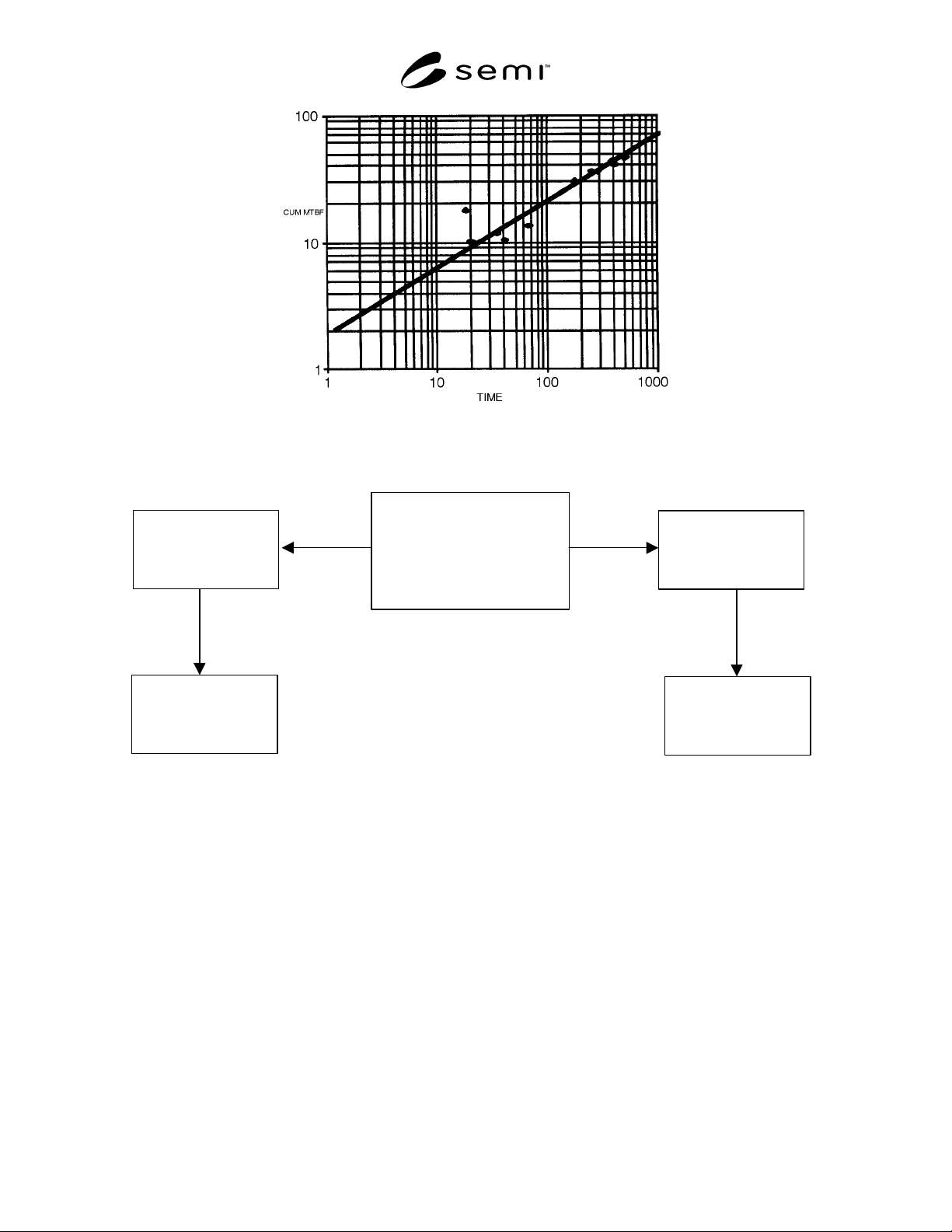
is likely. Figure A2-1 shows the Duane plot, which

appears to show a linear improvement trend on log-log

paper. The AMSAA model equations give an

improvement slope estimate of 0.43 and an

instantaneous MTBF

estimate at 550 hours of 87.2.

Note that a standard calculation ignoring the

improvement trend

would yield an MTBF

estimate of

550/11 = 50, which is a 43% underestimate.

A2-2.13 Figure A2-2 summarizes the recommended

procedure to follow when analyzing system or

equipment reliability data, with appropriate references

to SEMI E10 sections or appendices.

A2-3 References

1. Ascher, H. and H. Feingold, Repairable Systems

Reliability, Marcel Dekkar, Inc., New York, 1984

2. Tobias, P.A. and D.C. Trindade, Applied

Reliability, Second Edition, Van Nostrand

Reinhold, Inc., New York, 1995

3. Kendall, M.G., “A New Measure of Rank

Correlation”, Biometrika, 1938, volume 30, pages

81-93

4. Mann, H.B., “Nonparametric Test Against Trend”

Econometrica, 1945, volume 13, pages 245-25

5. Duane, J.T., “Learning Curve Approach to

Reliability Monitoring,” IEEE Transactions on

Aerospace, 1964, volume 2, pages 563-566

6. Crow, L.H., “Reliability Analysis for Complex

Repairable Systems,” Reliability and Biometry, F.

Proschan and R.J., Serfling, eds., SIAM,

Philadelphia, 1974; pp. 126-134

SEMI E10-0304

Figure A2-1

Duane Plot of CUM MTBF

vs. Time

Trend

o Trend

Sections 8.1-8.3/Appendix 2

Estimate the achieved

MTBF

at the end of

the period

Sections 6.2.1-6.2.2

Use standard MTBF

definition

Section 7.6/Appendix 1

Compute confidence

bounds for MTBF

Analyze the data for trends

Duane Plots

Trend Test

Section 8.3/Appendix 2

Fit AMSAA model

Figure A2-2

Flow Chart for Reliability Data Analysis

NOTICE: SEMI makes no warranties or representations as to the suitability of the standards set forth herein for any

particular application. The determination of the suitability of the standard is solely the responsibility of the user.

Users are cautioned to refer to manufacturer’s instructions, product labels, product data sheets, and other relevant

literature respecting any materials mentioned herein. These standards are subject to change without notice.

The user’s attention is called to the possibility that compliance with this standard may require use of copyrighted

material or of an invention covered by patent rights. By publication of this standard, SEMI takes no position

respecting the validity of any patent rights or copyrights asserted in connection with any item mentioned in this

standard. Users of this standard are expressly advised that determination of any such patent rights or copyrights, and

the risk of infringement of such rights, are entirely their own responsibility.