semi合集-English.pdf - 第7531页
SEMI MF1771-0304 © SEMI 2003, 2004 8 () () () ( ) () − − − − − 5 1 5 1 abs ln abs n V n V n I n I (5) while the new slope is comp uted from …
SEMI MF1771-0304 © SEMI 2003, 2004 7
all corrections indicated in Equation 3 must be taken
into account.
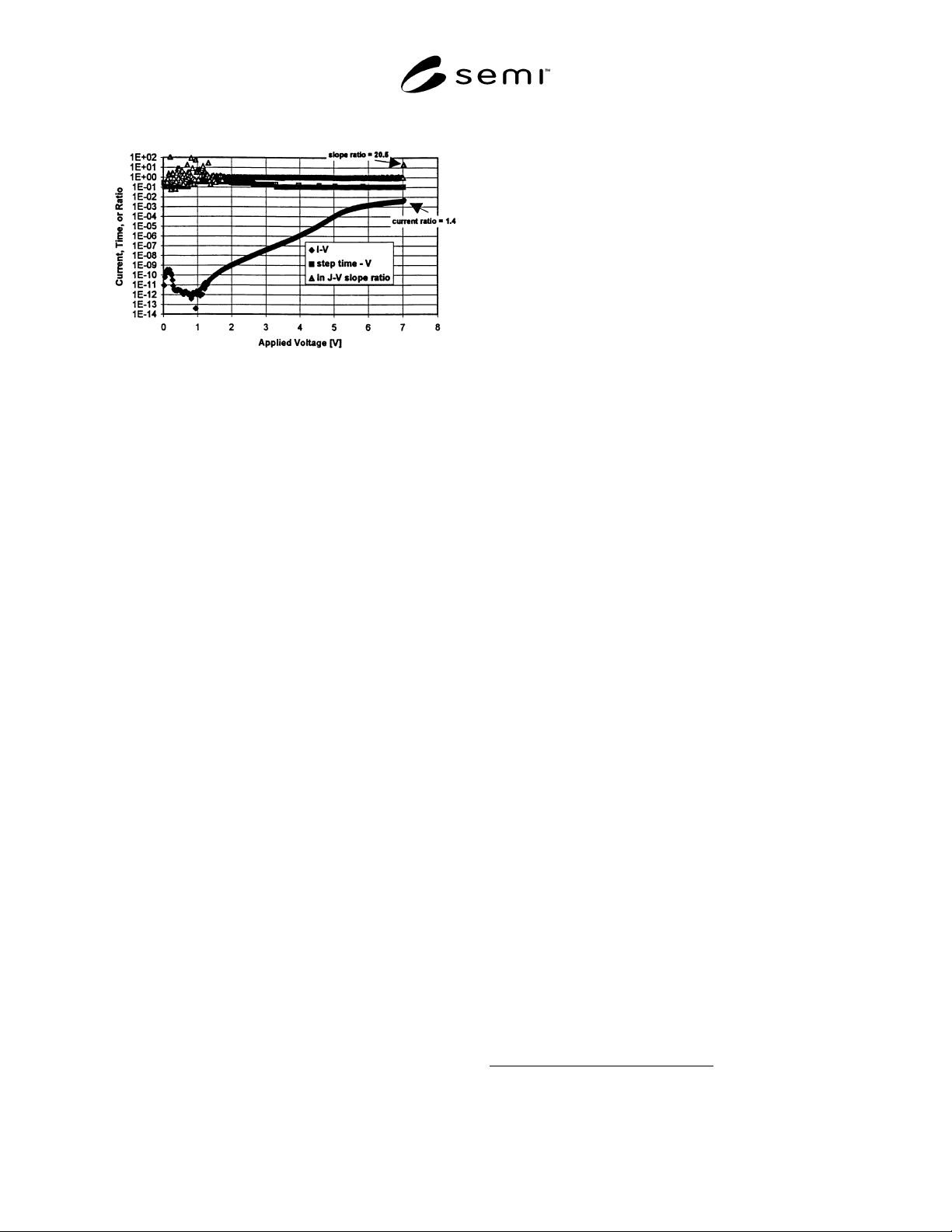
Figure 2
Determination of Noise Threshold Current Level,
Slope Ratio Applicability, and Voltage Step Time
Variations
10.3 Determination of Noise Threshold Current Level
and ln J-V Slope Ratio Specification — Useable values
of noise threshold current level and ln J-V slope ratio
depend upon properties of the test system as well as the
samples to be evaluated, and a preliminary test may be
required in order to specify them properly. To do this,
it is necessary to store all the current-voltage data pairs
as well as the incremental voltage step time readings in
data arrays. This is not required for performance of the
bulk of the testing, but is sometimes useful for more
thorough analysis of the test results. When such data is
stored, it is possible to construct a figure like that
shown in Figure 2, which is a semi-logarithmic plot of
sample current, step time, and slope ratio versus applied
voltage. Data given here was taken on a 3-nm oxide on
a p-type silicon substrate, so the current and voltage
values are magnitudes of negative readings. Both direct
and Fowler-Nordheim tunneling components are seen
in the I-V data.
10.3.1 To determine the noise threshold current level,
examine the ln J-V slope ratio, shown as open triangles
in Figure 2. It is seen to be quite noisy for this test
system and sample up to a current level just below 1
nA. This value, 1 nA, is thus a good choice for noise
threshold current level for this test. Further analysis of
the slope ratio data shows that its maximum value in the
range from 1 nA up to catastrophic failure is 1.21, so
the standard specified ratio value of three (3) is
adequate to avoid significant noise interference.
10.3.2 The step time-voltage dependence plotted as
light squares in Figure 2 illustrates shortcomings in the
step time control for this configuration of the
measurement system. A voltage step time of 0.1 s is
specified for this test method in Sections 5.3 and 9.7.
Because of the high, time-dependent currents measured
below 0.5 V, there is a regime below 1 V where this is
observed, but most readings from there up to a current
value of 0.1 µA fall in the range 0.2 to 0.4 s. Also, for
higher current values, there are singular points at
electrometer range changes where 0.2-s delays are
encountered. It has been shown (Klema
4
) that
deviations of this amount do not have large effects on
breakdown voltage distributions, but these extended
delays affect total measurement time, and it would be
worthwhile to eliminate them if possible. Approaches
depend upon measurement hardware being used, but
trading off low current resolution for electrometer
autoranging time and look-ahead range changing code
are possibilities.
10.4 ln J-V Slope Hard Failure Criterion — Hard
breakdown failure of oxides is increasingly difficult to
detect as oxide thickness decreases below 10 nm.
Fowler-Nordheim emission, the dominant current
transport mechanism for SiO
2
films in this thickness
range, predicts that at a given field strength, the
logarithmic slope of the J-V characteristic increases for
decreasing film thickness, but decreases with increasing
field strength for a given oxide thickness. Thus, a
change in ln J-V slope may be a more sensitive detector
of failure for these very thin films, where high failure
current density, low oxide impedance at failure, and
high voltage drops in series resistances might lead to
very small current changes when the oxide ruptures.
10.4.1 Experience with this failure criterion for oxide
thicknesses ranging down to 3 nm indicates that a
change by a factor of 3 provides good detection of
failure while remaining above the noise level in the
data. Users may verify this condition for their
particular sample and test conditions, and change the
failure factor accordingly. Any such change must be
agreed upon by the parties to the test, and clearly
identified in the report of the data.
10.4.2 In order to minimize noise in the calculated
values and optimize the sensitivity of the failure
detection, it has been found advisable to use a set of
five data points to calculate the established and new
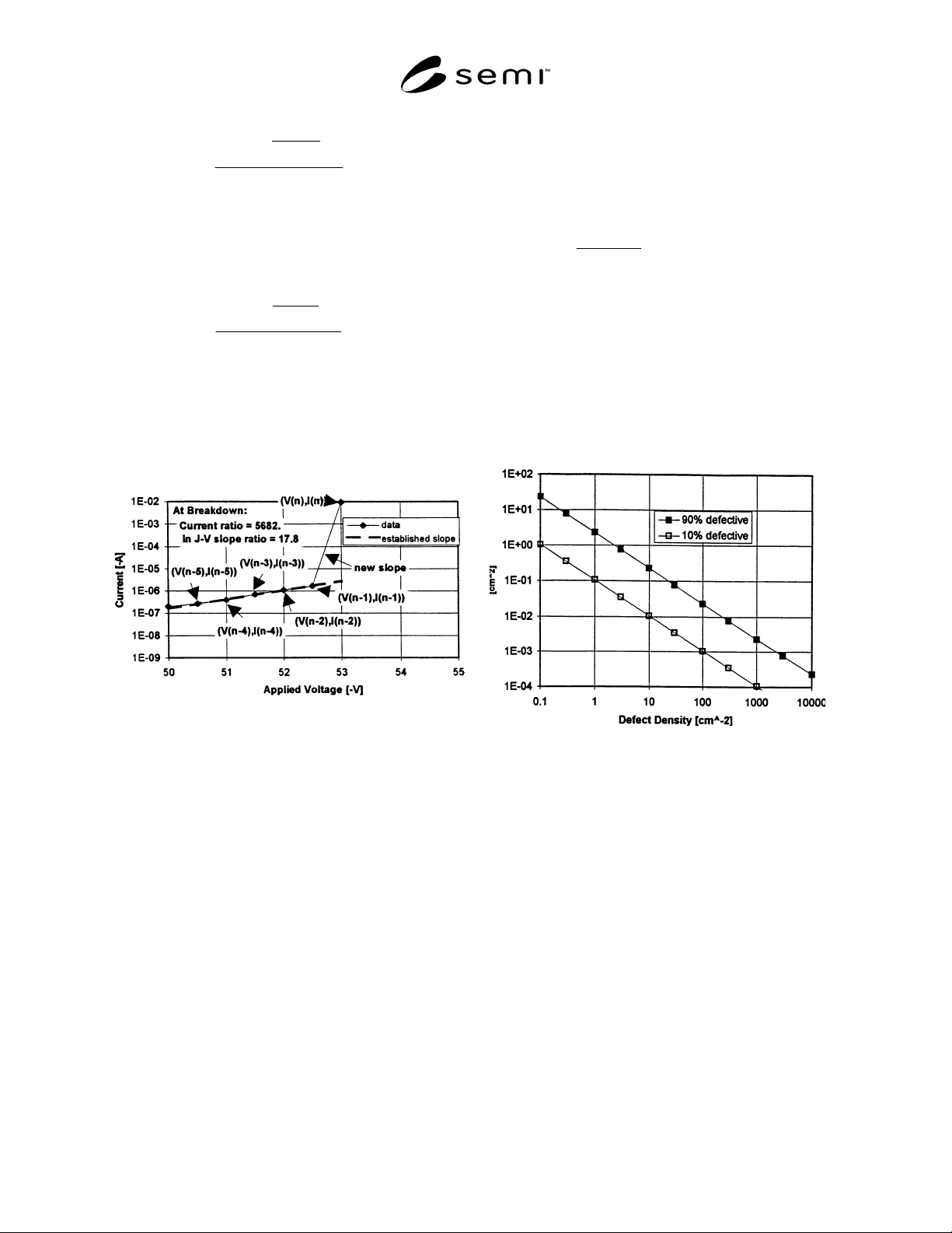
values of the ln J-V slope. This illustrated in Figure 3,
which shows the last few data points in the ramp
voltage test of a 50-nm oxide. Data points are spaced at
0.1 MV/cm increments, as dictated by this test method.
10.4.3 In particular, the last five data points are labeled
(V(n), I(n)) through (V(n – 5), I(n – 5), respectively.
The established logarithmic slope is as follows:
4 Klema, J., “Ramp Rate Effect on Dielectric Breakdown,” Final
Report, IEEE International Integrated Reliability Workshop (IRW),
IEEE Electron Devices Society, 1989, p. 87.
SEMI MF1771-0304 © SEMI 2003, 2004 8
()
()
()( )()
−−−
−
−
51
5
1
absln
abs
nVnV
nI
nI
(5)
while the new slope is computed from the last two
points,
()
()
() ( )()
−−
−
1
1
absln
abs
nVnV
nI
nI
(6)
10.4.4 Testing for the failure criterion is done by taking
the ratio of Equation 6 to Equation 5. As can be seen
from Figure 3, this failure would be identified by failure
criteria Sections 9.9.2 and 9.9.3, as well as the slope
criterion Section 9.9.5.
Figure 3
Calculation of In J-V Slope Ratio Failure
Criterion for a p-Type Sample with 50-nm Gate
Oxide
10.5 Defect Density — To calculate a defect density, a
minimum criterion must be chosen by either the user or
negotiated with the user' s customer. This criterion can
take the form of a minimum breakdown voltage or
electric field strength, or a discontinuity in the
breakdown voltage distribution of the sample. Given
the fraction of devices reaching this criterion, the defect
density calculation may be based on a Poisson
relationship (see Standard 35) using the following
equation:
)exp( ADY −= (7)
where:
Y = yield of good units in terms of the defined
failure criterion,
A = area of sample, cm
2
, and
D = defect density, defects/cm
2
.
NOTE 4: Example: Given a total of 100 devices tested with
87 devices passing the minimum criterion for success and a
gate area of 0.08 cm
2
, the defect density would be as follows:
2
defects/cm7.1
08.0
)100/87ln(
==D
(8)
10.5.1 An undefined condition results if the number of
successes is zero. It may be necessary to change the
area of the test capacitor chosen for testing in order to
resolve meaningful defect densities. Figure 4 shows the
relationship between defect density and test capacitor
area required for resolution in terms of a minimum of
10% good or defective units in the sample.
NOTE 5: For example, a test capacitor with an area of 0.1
cm
2
can resolve defect densities between 1 and 25
defects/cm
2
, with 10 and 90% defective samples.
Figure 4
Test Capacitor Area Required to Resolve Various
Oxide Defect Densities, Assuming Poisson Statistics
10.6 Weibull Distributions — To convert cumulative
percentages to Weibull format (sometimes referred to
as “smallest extreme value probability distribution III”),
use the following equation:
(
)
)1ln(ln F
−
−
(9)
where ln is the natural log operator and F is the fraction
of accumulated failures. Care should be taken so that F
is never exactly 1 since this results in an undefined
situation.
SEMI MF1771-0304 © SEMI 2003, 2004 9
11 Report
11.1 Report the following for each wafer, as
appropriate for the test conditions and as agreed upon
by the parties to the test:
11.1.1 Test Description:
11.1.1.1 Date,
11.1.1.2 Time,
11.1.1.3 Operator,
11.1.1.4 Instrument station identity (if any),
11.1.1.5 Test temperature, and
11.1.1.6 Total number of devices tested.
11.1.2 Sample Description:
11.1.2.1 Average oxide thickness,
11.1.2.2 Gate area, cm
2
,
11.1.2.3 Gate material,
11.1.2.4 Oxide type (example thermal versus
deposited),
11.1.2.5 Structure type,
11.1.2.6 Conductivity type (n or p),
11.1.2.7 Bias mode (accumulation or depletion), and
11.1.2.8 Average computed series resistance (R
s
), if
performed.
11.1.3 Test Results:
11.1.3.1 Medians and means for the hard and soft
breakdown voltage distributions (V
BD
) and the current
densities at breakdown (J
BD
),
11.1.3.2 Histograms of the hard and soft breakdown
voltage and breakdown current density data. These
results may also be presented in Weibull plot format,
11.1.3.3 Percentage of devices falling into each failure
mode category by hard or soft failure voltage, or by
oxide electric field. Include results of the post-test for
each category, and
11.1.3.4 Defect densities computed as described in
Section 10.5, and as agreed upon by participating
parties.
NOTE 6: For homogenous groups, data can be combined for
the purposes of comparison.
12 Precision and Bias
12.1 At this time, precision has not been established. A
reproducibility test for the similar Standard 35 has been
reported.
5
13 Keywords
13.1 current density; defect density; electric field
strength; extrinsic breakdown; intrinsic breakdown;
oxide breakdown
5 Suehle, John S., “Reproducibility of JEDEC Standard Current and
Voltage Ramp Test Procedures for Thin-Dielectric Breakdown
Characterization,” Final Report, IEEE International Integrated
Reliability Workshop (IRW), IEEE Electron Devices Society, 1993,
pp. 22–34.