semi合集-English.pdf - 第5812页
SEMI P24-94 © SEMI 1994, 2004 3 6 Procedures to Benchmark Precision 6.1 Precision Types 6.1.1 Static Precision — A series of measure ments made of a single feature where, for eac h measurement, the information is reacqui…
SEMI P24-94 © SEMI 1994, 2004 2
5 Terminology
5.1 Definitions
5.1.1 precision — the degree of agreement of repeated
measurements of the same parameter expressed
quantitatively as the standard deviation, computed from
the results of a series of controlled determinations
[ASTM D 1129, D-29].
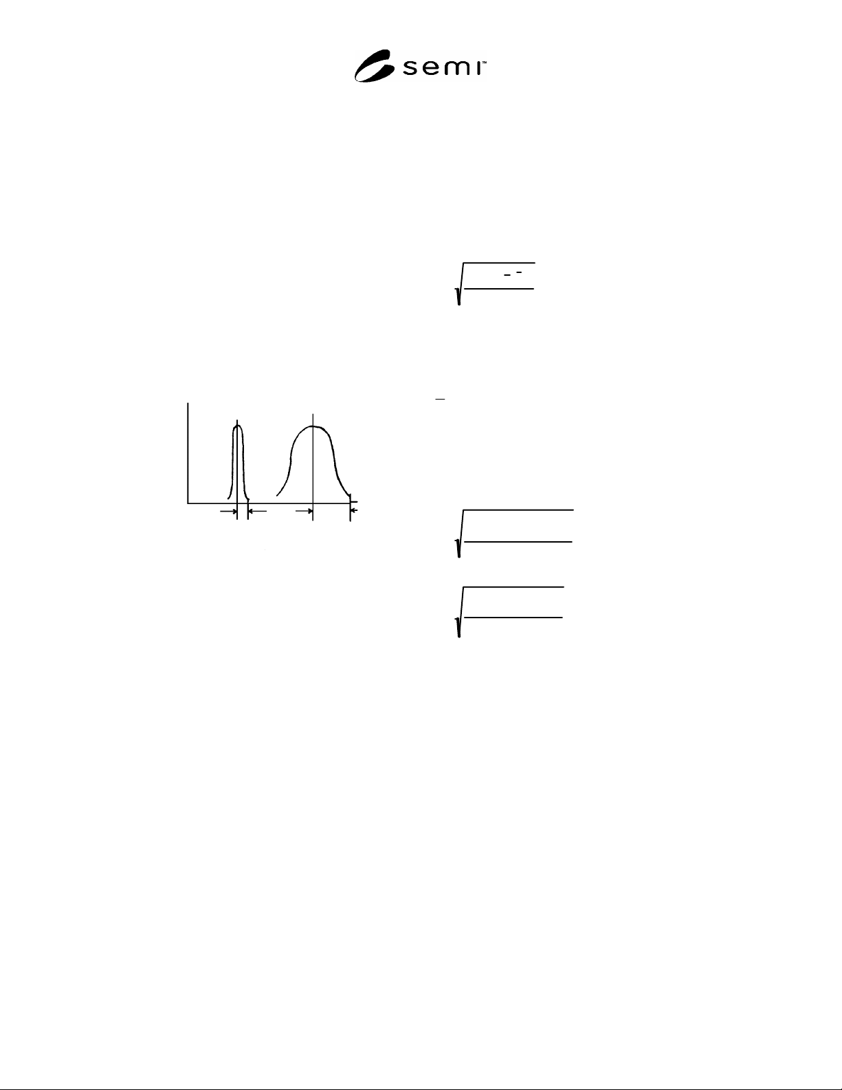
5.1.2 A frequency plot of measurements taken with
random error illustrates precision. The spread or
variation of measurement in test A is smaller than that
in test B. The results of test A are more precise than the
results from test B. See Figure 1.
NOTE 2: Any test procedure used needs to differentiate
between system and wafer contribution.
Frequency
Measurement
S
A
S
B
Figure 1
Generic Frequency Plot
5.1.3 repeatability — the standard deviation of results
obtained by the same operator using the same
instrument in successive measurements [ASTM C 609,
C-21]. The same system parameters need to be used.
The degree to which the individual operator affects the
measured result is a critical parameter and must be
identified and benchmarked.
NOTE 3: The degree to which the individual operator affects
the measured result may be a critical parameter and must be
identified.
5.1.4 reproducibility — the precision of a test method
expressed in terms of agreement expected between
measurements made in different laboratories using
similar apparatus and the same procedure [ASTM D
4790, D-16].
5.1.5 stability — the standard deviation of means of
groups of measurements taken at specified intervals
over an extended period of time.
NOTE 4: The means are used to avoid including the
measurement precision. Stability is a characterization of the
system independent of precision. It is important to use a stable
sample so that system stability, independent of the sample, is
determined.
5.1.6 standard deviation — a measure of the dispersion
of a series of results around their average, expressed as
the square root of the quantity, obtained by adding the
squares of the deviations from the average of the results
and dividing by the number of observations minus one.
It is also the square root of the variance and can be
calculated as follows:
s
x
i
x
2
n 1
1
Where:
s = estimated standard deviation of the series of results
X
i
= each individual value
X = average (arithmetic mean) of all values, and
n = number of values
The following forms of this equation are more
convenient for computation, especially when using a
calculator:
s
x
2
x
2
/ n
n 1
2
or
s
nx
2
x
2
nn 1
3
where:
s = estimated standard deviation
x
2
sum of the squares of all the individual values
x
2
square of the total of the individual values,
and
n = number of values
NOTE 5: Care must be taken in using either of these
equations that a sufficient number of decimal places is carried
in the sum of the values and in the sum of their square so that
serious rounding errors do not occur. For best results, all
rounding should be postponed until after a value has been
obtained for s [ASTM E 180, E 15].

SEMI P24-94 © SEMI 1994, 2004 3
6 Procedures to Benchmark Precision
6.1 Precision Types
6.1.1 Static Precision — A series of measurements
made of a single feature where, for each measurement,
the information is reacquired and reprocessed. The
minimal intervention required to repeat the
measurement will be used. The standard deviation will
be calculated based on the sample data.
6.1.2 Z (Axis Adjustment) Precision — A series of
measurements is made of a single feature where it is
necessary to refocus before each measurement (without
intentional movement in the x and y axes before each
measurement). The standard deviation will be
calculated based on the sample data.
6.1.2.1 Dynamic Precision — Make one measurement
of grouped line and space features at n number of sites
on a focus/exposure matrix wafer, which includes
typical size and side wall angle variations. Remove the
wafer from the system, then reload and remeasure.
Compute the dynamic precision, 3s, by the double
sample method (see Section 8.1.3).
6.1.2.1.1 A total of 1 size × n sites × 2 repeates = 2n
measure-ments per wafer × 3 passes = 6n
measurements required.
6.1.2.1.2 10 is a minimum recommended value for n.
6.1.2.1.3 This may also be redone for different
thicknesses of lines to be measured and repeated for
each of the wafer types in the process.
7 Precision Test
7.1 Test Methods
7.1.1 Stability Test Method — Makes a group of five
measurements of a stable feature, such as etched
polysilicon, at the same position, daily. Any system
adjustment, maintenance, environment variation is
allowed, but noted. Recalibration is optional, but is
noted. Use a feature which doesn’t change over time,
or with repeated measurements. Plot the daily averages
on an individual control chart with control limits based
on the moving range of the daily averages.
7.1.2 Sequence Test Method — A series or sequence of
measurements is taken of the same physical location.
Any change between measurements determines the type
of precision tested.
7.1.3 Double Sample Test Method — Two
measurements are taken at separate times within the test
run at a number of different physical locations. A
series of sites is used which have: same nominal size,
same proximity of other features, similar side wall
angle, etc.
7.2 Test Duration
7.2.1 Short Term — No system calibration, adjustment,
or maintenance will be done. The period should be
short enough to minimize the effect of environmental
variations. See R1-1.
7.2.2 Long Term — Any system adjustments,
maintenance, environment variation is allowed. See
R1-2. Recalibration is optional.
7.2.3 Presentation of Results — Some information,
relative to the data, must be included to qualify the
results. Graphical representation of the data is
recommended.
7.2.3.1 The following must be included:
The estimated (1, 2, or 3) standard deviation(s),
Short or Long Term
Confidence interval (see Application Note A.3)
The number of measurements or sample size (n)
Describe the feature film and substrate film
Nominal or average measurement
Feature Type: line or space or hole, grouped or
isolated
The frequency of recalibration
Test identified as the type performed
7.2.3.1.1 Additional information which should also be
included, particularly with unusual conditions, are:
Metric units are recommended, such as nanometer
[nm] or micrometer [µm]
Feature characteristics, such as: sidewall angle,
wall profile, corner radius, materials, thickness,
index of refraction, edge waviness, edge roughness
Duration of the test
The sample frequency
Significant parameters such as operator, system
model, serial number, pertinent environmental
conditions, etc.

SEMI P24-94 © SEMI 1994, 2004 4
8 Related Documents
“ASTM Compilation of ASTM Standard Definitions,”
American Society for Testing and Materials, 100 Barr
Harbor Drive, West Conshohoken, PA 19428.
Nyyssonen, Dr. Robert D. Larrabee, “Submicrometer
Linewidth Metrology for the Optical Microscope,” (J.
of Research of National Bureau of Standards, Vol. 92,
No. 3, May/June 1987). National Institute of Standards
and Technology (NIST), Bldg. 202, Room 204,
Gaithersburg, MD 20899.
Dr. Robert D. Larrabee and Dr. Michael T. Postek,
“Precision, Accuracy, Uncertainty and Traceability and
Their Application to Submicrometer Dimensional
Metrology” (Solid-State Electronics, Vol. 36, No 5, pp
673-684, 1993).
SEMASPEC #91090709A-ENG, “Introduction to
Measurement Capabilities Studies,” SEMATECH,
Technology Transfer, 2706 Montopolis Drive, Austin,
TX 78741.