semi合集-English.pdf - 第5318页
SEMI M50-1104 © SEMI 2001, 2004 4 11.1.2 Date of test; 11.1.3 Manufacturer, m odel, serial number, an d software ve rsion of t he SSIS bei ng tested, 11.1.4 Description of the reference wafer used in the test. 11.1.5 Plo…

SEMI M50-1104 © SEMI 2001, 2004 3
repeat LLS events on the wafer, M
2
, is larger than 0.75
M
1
. Make certain that the conditions of Sections 8.1
and 8.1.1 are fulfilled for both wafer scans.
9.2 Scan the wafer a total of Z times to obtain CR,
FCR, and CFCR data (see NOTES 3 and 6). Record
each LLS event detected during the Z scans according
to its position P and size S.
NOTE 5: The two scans obtained in Sections 9.1 through
9.1.2 can be used as part of this data set, but the wafer must
remain on the scan stage during the entire set of Z scans to
perform the measurement sequence under repeatability
conditions.
10 Analysis
10.1 Initial Analysis
10.1.1 Determine the locations on the wafer where an
LLS event has been detected at least once by comparing
all recorded positions (within the constraint of the six-
sigma XY uncertainty) of the multiple scans as reported
by the SSIS. These locations, L
i
, with i = [1, 2, …,N]
represent the complete set of LLS events to be used in
the analysis. Each location is characterized by the
number of scans H
i
, in which the LLS event at that
position has been detected, and by the H
i
reported sizes
S
ih
, where h = [1, 2, …,H
i
], for the LLS event.
10.1.2 Consider those of the N events with H
i
= 1, (i.e.,
events seen only once) as false counts. Order these
events by decreasing size, S
i
. Index them by f = [1, 2,
...,F], with f = 1 representing the largest size and f = F
representing the smallest.
10.1.3 Consider those events that were seen at least
twice during the Z scans (H
i
2) to be true counts.
NOTE 6: The sequence of analysis steps given below is
intended to be representative and illustrative. The actual
algorithms used in the analysis software may differ from these
as long as the same result is achieved.
10.2 Analysis of True Counts
10.2.1 Determine the average size <S
i
> of each true
count (H
i
2) as follows:
i
H
h
ih
i
i
S
H
S
1
1
(1)
10.2.2 Calculate the size dependent capture rate,
CR(<S
i
>), for every true count as follows:
Z
H
SCR
i
i
)( (2)
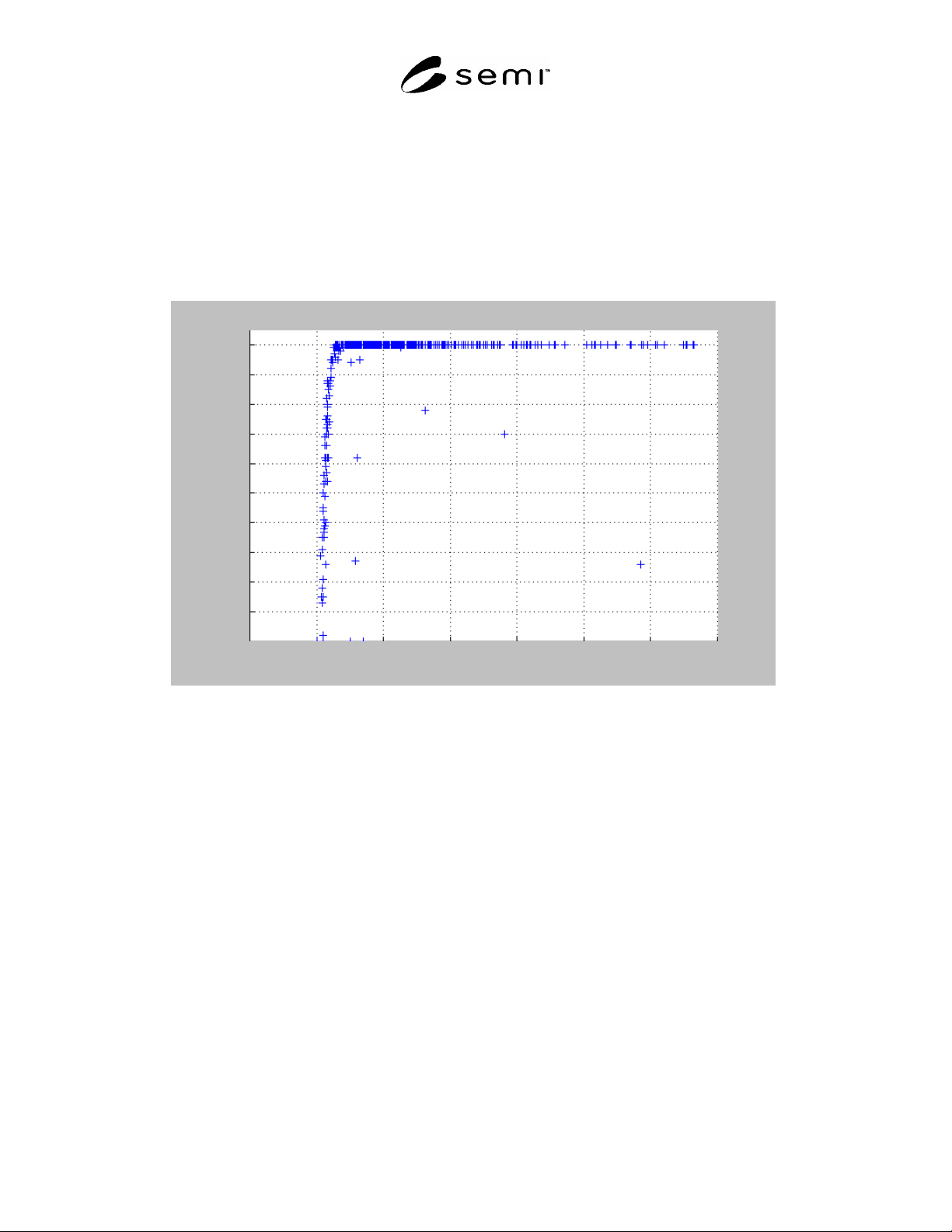
10.2.3 Plot CR(<S
i
>) versus <S
i
> as in the example in
Figure 1, and interpolate or fit the data to discriminate
against outlying points.
NOTE 7: The following equation for c
s,
in percent,
0
0
exp1100
c
ss
c
s
, (2a)
may be used to fit the plotted CR(<S
i
>) data. Here, c
s
is the
fitted value of CR(<S
i
>), s is the size (<S
i
>), s
0
is the size at
zero probability of capture, and c
0
is a curvature factor that
determines the point at which the probability of capture
approaches 100%. As c
0
and s
0
constitute a sufficient
parameter set to describe completely CR(<S
i
>), they can be
used for reporting, together with the chi-square goodness of
the fit test statistic result.
NOTE 8: Note that there are a few points below the principal
curve in Figure 1. These points may have arisen from added
particles that appeared on the wafer during the test. They
should be neglected in fitting any curve to the capture rate
data.
10.2.4 Calculate the standard deviation of size S
i
for all
true counts as follows:
i
H
h
iih
i
i
SS
H
S
1
2
)(
1
1
)(
(3)
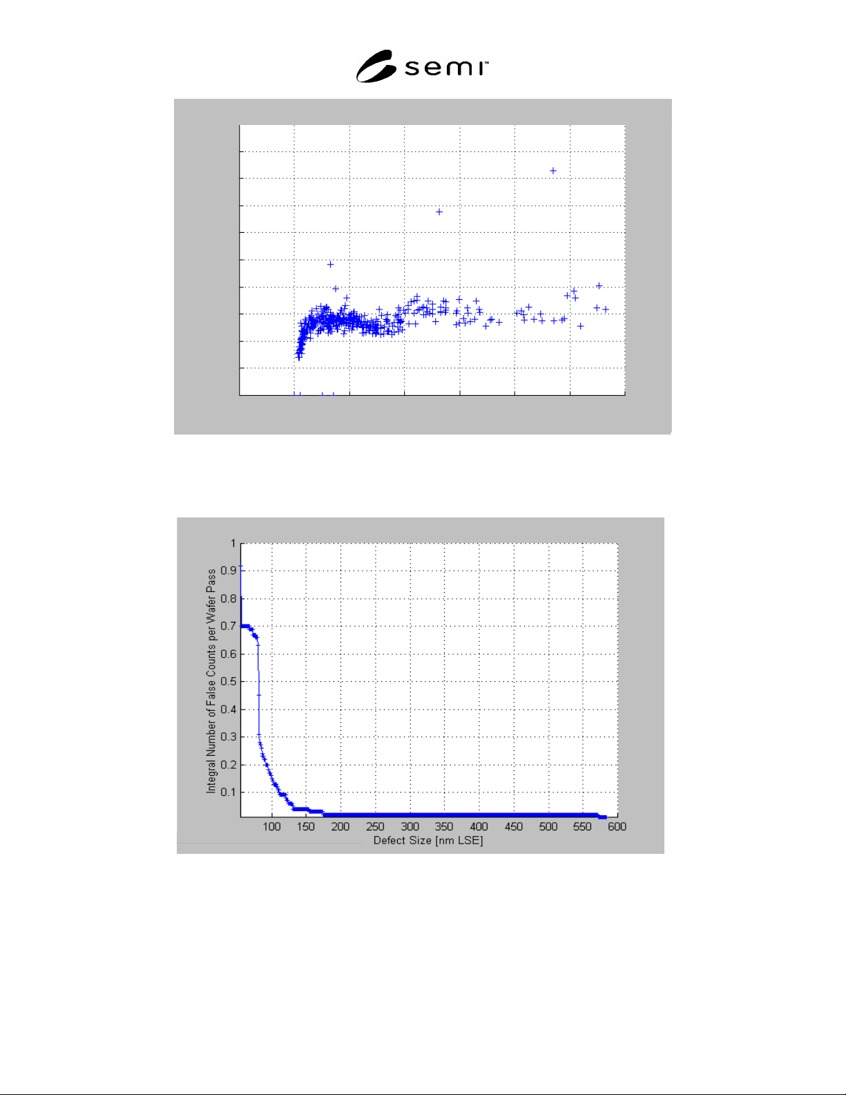
10.2.5 Plot the standard deviation of size, σ(S
i
), versus
the mean size, <S
i
>, for all true counts as shown in the
example in Figure 2.
NOTE 9: Again, note the same outliers in Figure 2. These
can be neglected in any analysis of the standard deviation
data.
10.3 Analysis of False Counts
10.3.1 Divide the total number of false counts, F, by
the number of scans, Z, to get the false count rate, FCR:
Z
F
FCR
(4)
10.3.2 Analyze the false count rate as a function of size
to determine the cumulative false count rate, CFCR(S
i
),
at each size, S
i
, by taking the total number of false
counts of size equal to or greater than S
i
, and dividing
by the number of scans, Z:
,)(
Z
F
SCFCR
i
i
(5)
where F
i
is the largest value of the index associated
with the count (or counts) of size S
i
.
10.3.3 Plot CFCR(S
i
) as a function of S
i
as shown in
the example in Figure 3.
11 Report
11.1 Report the following information:
11.1.1 Operator identification;
SEMI M50-1104 © SEMI 2001, 2004 4
11.1.2 Date of test;
11.1.3 Manufacturer, model, serial number, and
software version of the SSIS being tested,
11.1.4 Description of the reference wafer used in the
test.
11.1.5 Plot of the capture rate, CR(<S
i
>), vs. the mean
size, <S
i
>, similar to the example in Figure 1.
11.1.6 Plot of the standard deviation, (S
i
), of the LLS
mean size, <S
i
>, similar to the example in Figure 2.
11.1.7 Calculated false count rate, FCR, as described in
Section 10.3.2.
11.1.8 Plot of the cumulative false count rate,
CFCR(S
i
), similar to the example in Figure 3.
1
0.9
0.8
0.7
0.6
0.5
0.4
0.3
0.2
0.1
0
70 80 90 100 110 120 130 140
Mean Size <S
i
> of LLS [nm LSE]
Capture Rate CR (<S
i
>) [%/100]
NOTE 1: This figure is an example plot of capture rate as determined in Sections 10.2.1 through 10.2.3. The measurements in
this example are the result of 100 scans on a wafer with several natural LLS sites of different sizes. The SSIS noise floor was set
at 80 nm LSE.
Figure 1
Capture Rate
SEMI M50-1104 © SEMI 2001, 2004 5
5
4.5
4
3.5
3
2.5
2
1.5
1
0.5
0
70 80 90 100 110 120 130 140
Mean Size <S
i
> of LLS [nm LSE]
Standard Deviation of Size <S
i
> [nm LSE]
NOTE 1: This figure is an example plot of the standard deviation of true count size as determined in Sections 10.2.4 and 10.2.5.
Figure 2
Standard Size Deviation
0.0
50
NOTE 1: This figure is an example plot of cumulative false count rate as determined in Sections 10.3.1 through 10.3.3. This is
the same data set used for Figures 1 and 2; however, the horizontal scale has been expanded.
Figure 3
Cumulative False Count Rate (CFCR)