semi合集-English.pdf - 第860页

SEMI E115-0302 E © SEMI 2002 6 10.2 Report the m atching network load impedance an d e fficiency as a function of tu ning element positions . The data shall be presented in both graphical and tabular form s. 11 Related D…

SEMI E115-0302

impedance to vary. An example of a load simulator

would be a matching network used in reverse, where

the output of the DUT would attach to the output of

another matching network.

9.4.2 Calibrate the Network Analyzer at the desired

operating frequency (e.g., 13.56 MHz). The Network

Analyzer shall be calibrated for measuring the

reflection coefficient at test Port 1 and for measuring

the transmission coefficient at test Port 2 (see Figure 1)

using the calibration kit provided with the Network

Analyzer. This measurement requires measuring the

S11 and S21 S-parameters and requires a full 2-port

calibration. The calibration shall be performed at fixed

frequency (continuous-wave operation) using the

lowest bandwidth possible (typically 10 Hz). The

calibration for each port shall include the additional test

cables and any additional adapters.

9.4.3 After calibration of the Network Analyzer, the

test cable connected to Port 1 of the Network Analyzer

shall be connected to the input of the matching network

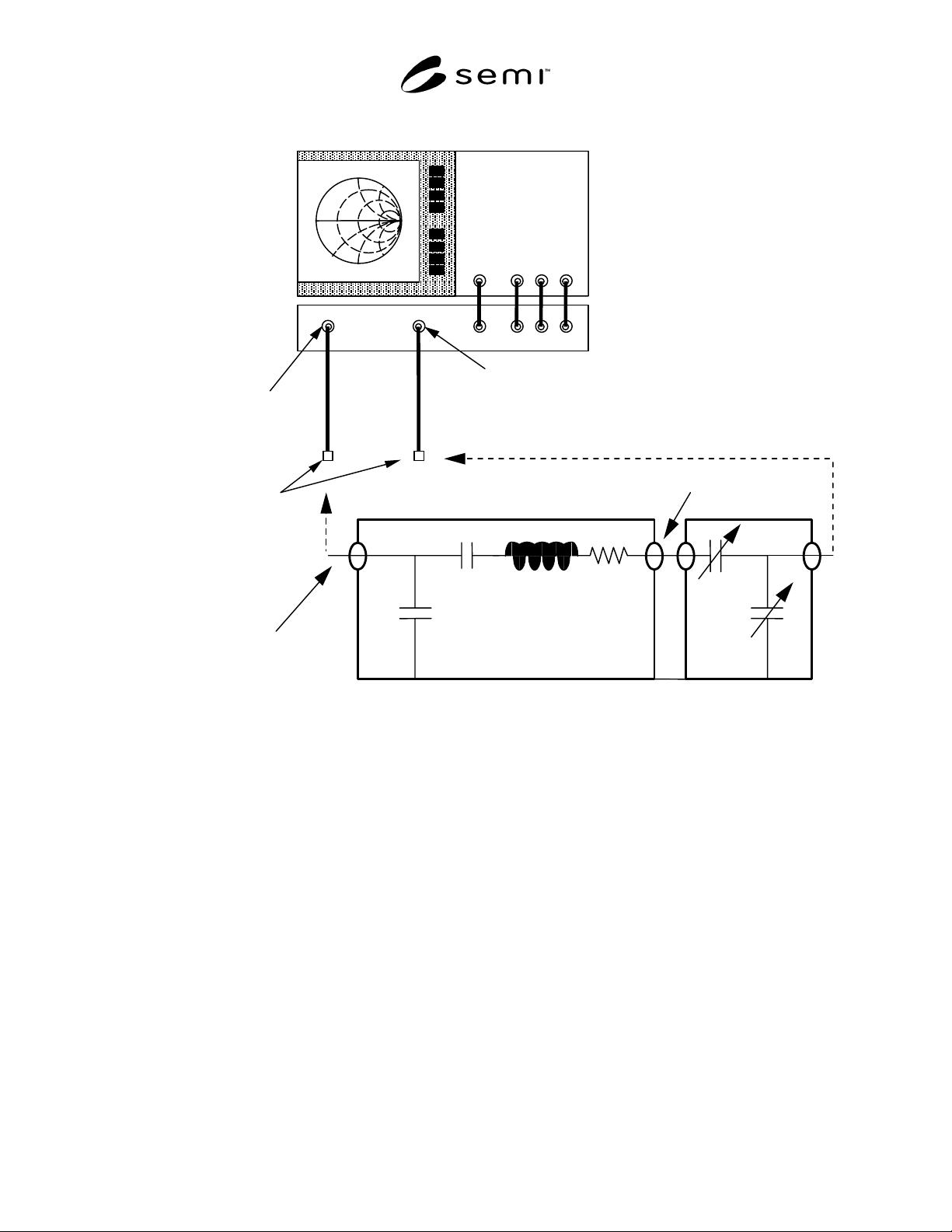
to be tested (DUT). The Load Simulator shall be

connected to the output of the DUT. The cable

connected to Port 2 of the Network Analyzer shall be

connected to the output of the Load Simulator.

9.4.4 The tuning elements shall be moved to their

minimum positions (or the positions that can match to

lowest tuning point of the Load Simulator(s)) before the

measurement is initiated. The variable elements in the

Load Simulator shall be adjusted until the input

impedance of the matching network is matched (i.e.,

input impedance = 50 ohms). After all connections are

visually inspected for proper contact and the Network

Analyzer has stabilized, the value of the input

impedance and the magnitude of the transmission

coefficient (S21) shall be recorded. In addition, the

positions of the tuning elements of the DUT and the

Load Simulator shall be recorded.

9.4.5 The load impedance of the DUT corresponds to

the input impedance of the Load Simulator. At this

point in the process, the Load Simulator can be

disconnected and its input impedance can be measured.

Alternatively, the input impedance can be measured

later by moving the Load Simulator tuning element

values to the positions recorded in Section 9.4.4.

9.4.6 The efficiency of the Test Setup, which includes

the DUT and the Load Simulator, is determined from

the transmission coefficient. Typically, the

transmission coefficient is expressed in terms of dB

(decibels). The conversion between dB and percentage

is expressed as:

Efficiency(%) = 100 × 10

(loss in dB

10)

For example, if the transmission coefficient is measured

to be –3 dB, then the power transfer efficiency would

be 50.1%. In other words, 49.9% of the power is lost in

the Test Setup.

9.4.7 The efficiency of the DUT is determined by

dividing the efficiency of the Test Setup by the

efficiency of the Load Simulator. For example, if the

efficiency of the Test Setup is 70% and the efficiency

of the Load Simulator is 90%, then the efficiency of the

DUT is 77.8% (0.7/0.9). The efficiency of the Load

Simulator is typically determined separately (see

Related Information Section at the end of this Test

Method).

9.4.8 For the next measurement, one tuning element

(element 1) shall remain fixed, and the other tuning

element (element 2) shall be increased by an increment

equal to no more than 10% of the full scale range of the

tuning element position. For example, if the range of

the tuning element is 10 volts, then the tuning element

shall be moved in increments of no greater than 1 volt.

A smaller increment shall be used for the case where

the incremental change in tuning element position

results in an incremental impedance change of more

than 20% of the total impedance variation measured by

the full-scale variation of the tuning element. For

example, if the real part of the load impedance varies

15 ohms over the 10 volt variation of the tuning

element, then a smaller tuning element increment shall

be used if the real load impedance varies by more than

3 ohms between increments (0.2 × 15 = 0.3). After the

tuning elements have been moved to their new values,

the previous measurement steps shall be repeated.

9.4.9 After the tuning element (element 2) has been

varied over its entire range, the other tuning element

(element 1) shall be increased by an increment equal to

no more than 10% of its full-scale range. Tuning

element 2 shall be moved back to its minimum position

and the above steps shall be repeated until the entire

tuning range of the matching network is measured.

9.4.10 The data shall be recorded and then presented in

both graphical and tabular forms. An example of a

typical impedance range graph is shown in Figure 3 for

the real load impedance and in Figure 4 for the reactive

load impedance. An example of a typical efficiency

plot is shown in Figure 5. An example of data

presented in tabular form is shown in Table 1.

10 Reporting Test Results

10.1 Report the type of Network Analyzer and the

details of the Network Analyzer parameters used for the

tests, including the bandwidth, the number of data

points, and the test frequency. Also report which Test

Method was used.

SEMI E115-0302

10.2 Report the matching network load impedance and efficiency as a function of tuning element positions. The

data shall be presented in both graphical and tabular forms.

11 Related Documents

11.1 IEEE Standards

IEEE-STD-572 — IEEE Standard for Qualification of Class 1E Connection Assemblies for Nuclear Power

Generating Stations

11.2 Military Standards

MIL-PRF-31031A — General Specification for Connectors, Electrical, Plugs and Receptacles, Coaxial, Radio

Frequency, High Reliability, for Flexible and Semirigid Cables.

MIL-STD-348 — General Specification for Radio Frequency Connector Interfaces.

MIL-STD-220B — Test Method Standard: Method of Insertion Loss Measurement.

RF out R

Port 2Port 1

Port 1

RLOSS

LC2

Input Connection

Output Connection

Matching Network

Port 2

Perform Calibrations

at End of Additional

Test Cables

Network

Analyzer

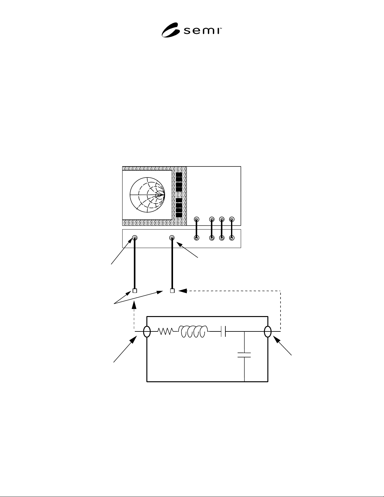
NOTE 1: Both the Port 1 and Port 2 outputs need to be used for the measurement. Additional test cables are needed for the

transmission calibration between the two ports. The output connection of the matching network to be tested (DUT) attaches to

Port 1 and the input connection of the matching network attaches to Port 2 of the Network Analyzer.

Figure 1

Schematic of the Test Method 1 Network Analyzer Test Setup for the Load Impedance and Efficiency

Measurement for “L” Type Matching Networks

SEMI E115-0302

RF out R

Port 2Port 1

Port 1

Port 2

Perform Calibrations

at End of Additional

Test Cables

RLOSS

LC2

Load Simulator

Input Connection

Output Connection

Matching Network

Network

Analyzer

NOTE 1: Both the Port 1 and Port 2 outputs need to be used for the measurement and additional test cables are needed for the

transmission calibration between the two ports. The input connection of the matching network to be tested (DUT) attaches to

Port 1, the output connection of the matching network attaches to the input of the Load Simulator, and the output of the Load

Simulator attaches to Port 2 of the Network Analyzer.

Figure 2

Schematic of the Test Method 2 Network Analyzer Test Setup for the Load Impedance and Efficiency

Measurement